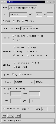
Figure 2: Control panel for the xflash visualization tool under IDL.
This section describes how to quickly get up and running with FLASH, showing how to configure and build it to solve the Sedov explosion problem, how to run it, and how to examine the output using IDL. To begin, verify that you have the following:
FLASH has been tested on the following Unix-based platforms. In addition, it may work with others not listed (see section ).
In this section we will use irix as an example of the machine type. Substitute your machine type for irix wherever it appears.
To begin, unpack the FLASH source code distribution. If you have a Unix tar file, type `tar xvf FLASHX.tar' (without the quotes), where X is the FLASH major version number (for example, use FLASH1.tar and FLASH1/ for FLASH version 1.0). If you are working with a CVS source tree, use `cvs checkout FLASHX' to obtain a personal copy of the tree. You may need to obtain permission from the local CVS administrator to do this. In either case you will create a directory called FLASHX/. Type `cd FLASHX' to enter this directory.
Next, configure the FLASH source tree for the Sedov explosion problem. Type
./setup sedov irix -defaults
This configures FLASH for the sedov problem, using the default hydrodynamic solver, equation of state, and I/O format defined for this problem. The source tree is configured to create a two-dimensional code by default.
The next step is to edit the file object/Makefile.h. This file contains all of the site-dependent and architecture-dependent parts of the Makefile. Verify that the compiler settings (FCOMP, CCOMP, and CPPCOMP) and the library paths (LIB) are correct for your system. No other changes should be necessary at this stage (later on you may wish to fiddle with the compiler optimization settings). Future versions of FLASH may make use of the GNU configure program to handle this step.
From the FLASH root directory (ie. the directory from which you ran setup), execute make. This will compile the FLASH code. If you should have problems and need to recompile, `make clean' will remove all object files from the object/ directory, leaving the source configuration intact; `make realclean' will remove all files and links from object/. After `make realclean,' a new invocation of setup is required before the code can be built.
Assuming compilation and linking were successful, you should now find an executable named flashX_sedov_irix in the object/ directory. (Remember to replace irix with your machine type.) You may wish to check that this is the case.
FLASH expects to find a flat text file named flash.par in the directory from which FLASH is run. This file sets the values of various runtime parameters which determine the behavior of FLASH. If it is not present, FLASH will use default values for the runtime parameters, which may or may not produce desirable results. Here we will create a simple flash.par which sets a few parameters and allows the rest to take on default values. With your text editor, create flash.par in the main FLASH directory with the contents of Figure .
# runtime parameterslrefine_max = 4
basenm = ßedov_4_"
restart = .false.
trstrt = 0.005
nend = 1000
tmax = 0.02
gamma = 1.4
xlboundary = -21 # code -21 is outflow
xrboundary = -21
ylboundary = -21
yrboundary = -21
This instructs FLASH to use up to four levels of adaptive mesh refinement (AMR) and to name the output files appropriately. We will not be starting from a checkpoint file (this is the default, but here it is explicitly set for purposes of illustration). Output files are to be written every 0.005 time units, and we will integrate until t = 0.02 or 1000 timesteps have been taken, whichever comes first. The ratio of specific heats for the gas (g) is taken to be 1.4, and all four boundaries of the two-dimensional grid have outflow (zero-gradient or Neumann) boundary conditions. Note the format of the file: each line is a comment (denoted by a hash mark, #), blank, or of the form variable = value. String values are enclosed in double quotes ("). Boolean values are indicated in the Fortran style, .true. or .false.
We are now ready to run FLASH. To run FLASH on N processors, type
mpirun -np N object/flashX_sedov_irix
remembering to replace N, X, and irix with the appropriate values. Some systems may require you to start MPI programs with a different command; use whichever command is appropriate to your system. The FLASH executable can take one command-line argument, the name of the runtime parameter file. The default parameter file name is flash.par.
You should see a number of lines of output indicating that FLASH is initializing the Sedov problem, listing the initial parameters, and giving the timestep chosen at each step. At the end FLASH prints a summary of the CPU time spent in various parts of the code and terminates. In the current directory you should now find several files:
We will use the xflash routine under IDL to examine the output. Before doing so, we need to set the values of two environment variables, IDL_PATH and XFLASH_DIR. Under csh this can be done using the commands
setenv XFLASH_DIR "$PWD/tools/idl"
setenv IDL_PATH "${XFLASH_DIR}:$IDL_PATH"
If you get a message indicating that IDL_PATH is not defined, just enter
setenv IDL_PATH "$XFLASH_DIR"
Now run IDL (idl) and enter xflash at the IDL> prompt. You should see a control panel widget as shown in Figure .
The path entry should be filled in for you with the current directory. Enter sedov_4_ as the base filename and enter 4 as the suffix. (xflash can generate output for a number of consecutive files, but if you fill in only the beginning suffix, only one file is read.) Our output files are in HDF format, so make sure the HDF button is selected. Choose the image format (screen, Postscript, GIF) and the problem type (in our case, Sedov). Selecting the problem type is only important for choosing default ranges for our plot; plots for other problems can be generated by ignoring this setting and overriding the default values for the data range and the coordinate ranges. Select the desired plotting variable and colormap. The `abundance conservation' variable produces a plot of the sum of the nuclear abundances, useful for comparison with the expected value (unity). Under `Options,' select whether to plot the logarithm of the desired quantity, and select whether to plot the outlines of the AMR blocks. For very highly refined grids the block outlines can obscure the data, but they are useful for verifying that FLASH is putting resolution elements where they are needed. Finally, check `velocity vectors' to overlay the velocity field. The `xskip' and `yskip' parameters enable you plot only a fraction of the vectors so that they do not obscure the background plot.
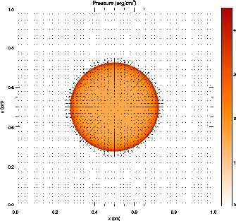
When the control panel settings are to your satisfaction, click the `Plot' button to generate the plot. For Postscript and GIF output, a file is created in the current directory. The result should look something like Figure 3, although this figure was generated from a run with eight levels of refinement rather than the four used in the quick start example run. With fewer levels of refinement the Cartesian grid causes the explosion to appear somewhat diamond-shaped.
FLASH is intended to be customized by the user to work with interesting initial and boundary conditions. In the following sections we will cover in more detail the structure of FLASH and the sample problems and tools distributed with it.
![]() Go on to Section 4.
Go on to Section 4.