Contents

Acknowledgments

The FLASH Code Group is supported by the (ASC) Flash Center at the University of Chicago under U. S. Department of Energy contract B341495. Some of the test calculations described here were performed using the Origin 2000 computer at Argonne National Laboratory and the (ASC) Blue Mountain computer at Los Alamos National Laboratory.

1  Introduction

The Center for Astrophysical Thermonuclear Flashes, or Flash Center, was founded at the University of Chicago in 1997 under contract to the United States Department of Energy as part of its Accelerated Strategic Computing Initiative ((ASC)). The goal of the Center is to solve several problems related to thermonuclear flashes on the surfaces of compact stars (neutron stars and white dwarfs), in particular X-ray bursts, Type Ia supernovae, and novae. To solve these problems requires the participants in the Center to develop new simulation tools capable of handling the extreme resolution and physical requirements imposed by conditions in these explosions, and to do so while making efficient use of the parallel supercomputers developed by the ASC project, the most powerful constructed to date.

The FLASH code (Fryxell et al. 2000) represents an important step along the road to this goal. FLASH is a modular, adaptive, parallel simulation code capable of handling general compressible flow problems in astrophysical environments. FLASH has been designed to allow users to configure initial and boundary conditions, change algorithms, and add new physical effects with minimal effort. It uses the PARAMESH library to manage a block-structured adaptive grid, placing resolution elements only where they are needed most. FLASH uses the Message-Passing Interface (MPI) library to achieve portability and scalability on a variety of different message-passing parallel computers.

This user's guide is designed to enable individuals unfamiliar with the FLASH code to quickly get acquainted with its structure and to move beyond the simple test problems distributed with FLASH, customizing it to suit their own needs. Section 2 discusses how to quickly get started with FLASH, describing how to configure, build, and run the code with one of the included test problems, then examine the resulting output. Users familiar with the capabilities of FLASH who wish to quickly `get their feet wet' with the code should begin with this section.

Section 3 describes the equations and algorithms used by the physics modules distributed with FLASH. It assumes that the reader has some familiarity both with the basic physics involved and with numerical hydrodynamics methods. This familiarity is absolutely essential in using FLASH (or any other simulation code) to arrive at meaningful solutions to physical problems. The novice reader is directed to an introductory text, examples of which include

       Fletcher, C. A. J. Computational Techniques for Fluid Dynamics (Springer-Verlag, 1991)

       Laney, Culbert B. Computational Gasdynamics (Cambridge UP, 1998)

       LeVeque, R. J., Mihalas, D., Dorfi, E. A., and Müller, E., eds. Computational Methods for Astrophysical Fluid Flow (Springer, 1998)

       Roache, Patrick. Fundamentals of Computational Fluid Dynamics (Hermosa, 1998)

Section 4 describes in more detail the use of the configuration and analysis tools distributed with FLASH. Section 5 describes the different test problems distributed with FLASH. The sixth section describes the FLASH code structure at length and gives detailed instructions for extending FLASH's capabilities by adding new problem setups. This section also discusses the code modules included with FLASH 1.6 and describes how new solvers may be integrated into the code. Finally, the seventh section gives guidance on contacting the authors of FLASH.

2  Quick start

This section describes how to quickly get up and running with FLASH, showing how to configure and build it to solve the Sedov explosion problem, how to run it, and how to examine the output using IDL. To begin, verify that you have the following:

• A copy of the FLASH source code distribution. This is most likely available either as a Unix tar file or as a local Concurrent Versions System (CVS) source tree. To request a copy of the distribution, click on the ``Code Request'' link at the Flash Code Group web site, http://flash.uchicago.edu/flashcode/. You will be asked to fill out a short form before receiving download instructions.
• A Fortran 90 compiler and a C compiler. Most of FLASH is written in Fortran 90. Information available at the Fortran Market web site (http://www.fortran.com/) can help you select a Fortran 90 compiler for your system.
• An installed copy of the Message-Passing Interface (MPI) library. A freely available implementation of MPI has been created at Argonne National Laboratory and can be accessed on the World Wide Web at http://www-unix.mcs.anl.gov/mpi/mpich/.
• If you plan to use the Hierarchical Data Format (HDF) for output files (the default), you will need an installed copy of the freely available HDF library. Currently FLASH supports HDF versions 4 and 5 (the two formats are not compatible). HDF is available from the HDF Project of the National Computational Science Alliance at http://hdf.ncsa.uiuc.edu/. The contents of HDF output files produced by the FLASH io/hdf* modules are described in detail in section 6.2.
• To use the output analysis tools described in this section, a copy of the IDL language from Research Systems, Inc. (http://www.rsinc.com/). IDL is a commercial product. It is not required for the analysis of FLASH output, but without it the user will need to write his or her own analysis tools. (FLASH output formats are described in Section 6.2.) The FLASH code group is currently working with members of the Mathematics and Computer Science Division at Argonne National Laboratory to develop more sophisticated visualization tools to distribute either as part of or alongside FLASH.
• The GNU make utility, gmake. This utility is freely available and has been ported to a wide variety of different systems. (For more information, see the entry for make in the development software listing at http://www.gnu.org/.) On some systems make is an alias for gmake. GNU make is required because FLASH 1.6 and higher uses macro concatenation when constructing Makefiles.

FLASH has been tested on the following Unix-based platforms. In addition, it may work with others not listed (see section 6.5).

• SGI single- and multiprocessor systems running IRIX
• Intel- and Alpha-based systems running Linux, including clusters
• Cray/SGI T3E running UNICOS
• The (ASC) Nirvana machine, built by SGI
• The (ASC) Blue Pacific machine, built by IBM
• The (ASC) Red machine, built by Intel

To begin, unpack the FLASH source code distribution. If you have a Unix tar file, type `tar xvf FLASHX.Y.tar' (without the quotes), where X.Y is the FLASH version number (for example, use FLASH1.61.tar and FLASH1.61/ for FLASH version 1.61). If you are working with a CVS source tree, use `cvs checkout FLASHX.Y' to obtain a personal copy of the tree. You may need to obtain permission from the local CVS administrator to do this. In either case you will create a directory called FLASHX.Y/. Type `cd FLASHX.Y' to enter this directory.

Next, configure the FLASH source tree for the Sedov explosion problem. Type

./setup sedov -defaults

If your system is not one of the configured sites (type ls source/sites for a list), or for some reason hostname does not return the correct site name, setup will attempt to locate your operating system type (determined via uname) in source/sites/Prototypes/. If this also does not succeed, you will need to do one of two things. If hostname or uname did not succeed, you can specify your site name or OS type using the -site or -ostype option to setup. Type ./setup without any options to see the syntax. If you are working on a new system with no available prototype, create a directory under source/sites with the name of your system (mkdir source/sites/`hostname`) and copy the file Makefile.h from a similar prototype directory to it. Then run ./setup sedov -defaults.

The next step is to edit the file object/Makefile.h. This file contains all of the site-dependent and architecture-dependent parts of the Makefile. Verify that the compiler settings (FCOMP, CCOMP, and CPPCOMP) and the library paths (LIB) are correct for your system. No other changes should be necessary at this stage (later on you may wish to fiddle with the compiler optimization settings). Future versions of FLASH will make use of the GNU configure program to handle this step.

From the FLASH root directory (ie. the directory from which you ran setup), execute gmake. This will compile the FLASH code. If you should have problems and need to recompile, `gmake clean' will remove all object files from the object/ directory, leaving the source configuration intact; `gmake realclean' will remove all files and links from object/. After `gmake realclean,' a new invocation of setup is required before the code can be built.

Assuming compilation and linking were successful, you should now find an executable named flashX in the object/ directory, where X is the major version number (e.g., X = 1 for X.Y = 1.61). You may wish to check that this is the case.

FLASH expects to find a flat text file named flash.par in the directory from which it is run. This file sets the values of various runtime parameters which determine the behavior of FLASH. If it is not present, FLASH will use default values for the runtime parameters, which may or may not produce desirable results. Here we will create a simple flash.par which sets a few parameters and allows the rest to take on default values. With your text editor, create flash.par in the main FLASH directory with the contents of Figure 1.

# runtime parameters lrefine_max = 4 basenm = ßedov_4_" restart = .false. trstrt = 0.005 nend = 1000 tmax = 0.02 gamma = 1.4 xlboundary = -21 # code -21 is outflow xrboundary = -21 ylboundary = -21 yrboundary = -21

This instructs FLASH to use up to four levels of adaptive mesh refinement (AMR) and to name the output files appropriately. We will not be starting from a checkpoint file (this is the default, but here it is explicitly set for purposes of illustration). Output files are to be written every 0.005 time units, and we will integrate until t=0.02 or 1000 timesteps have been taken, whichever comes first. The ratio of specific heats for the gas (g) is taken to be 1.4, and all four boundaries of the two-dimensional grid have outflow (zero-gradient or Neumann) boundary conditions. Note the format of the file: each line is a comment (denoted by a hash mark, #), blank, or of the form variable = value. String values are enclosed in double quotes ("). Boolean values are indicated in the Fortran style, .true. or .false.

We are now ready to run FLASH. To run FLASH on N processors, type

mpirun -np N object/flashX

You should see a number of lines of output indicating that FLASH is initializing the Sedov problem, listing the initial parameters, and giving the timestep chosen at each step. After the run is finished, in the current directory you should find several files:

• flash.log echoes the runtime parameter settings and indicates the run time, the build time, and the build machine. During the run, a line is written for each timestep, along with any warning messages. At the end of the run, a performance summary is written to this file.
• flash.dat contains a number of quantities as functions of time: total mass, total energy, total momentum, etc. This file can be used directly by plotting programs such as gnuplot; note that the first line begins with a hash (#) and thus is ignored by gnuplot.
• sedov_4_hdf_chk_000* are the different checkpoint files. These are complete dumps of the entire simulation at intervals of trstrt, suitable for use in restarting the simulation. They are also the primary output products of FLASH.
• sedov_4_hdf_plt_cnt_000* are plot files. These are files containing only density, temperature, pressure, and total energy (in single precision, for some I/O modules). They are designed to be written more frequently than checkpoint files for the purpose of making simulation movies (or for analyses that do not require all of the checkpointed quantities).

setenv XFLASH_DIR "$PWD/tools/idl"
setenv IDL_PATH "${XFLASH_DIR}:$IDL_PATH"

setenv IDL_PATH "$XFLASH_DIR"

The path entry should be filled in for you with the current directory. Enter sedov_4_hdf_chk_ as the base filename and enter 4 as the suffix. (xflash can generate output for a number of consecutive files, but if you fill in only the beginning suffix, only one file is read.) Click the `Discover Variables' button to scan the file and generate the variable list. Choose the image format (screen, Postscript, GIF) and the problem type (in our case, Sedov). Selecting the problem type is only important for choosing default ranges for our plot; plots for other problems can be generated by ignoring this setting and overriding the default values for the data range and the coordinate ranges. Select the desired plotting variable and colormap. Under `Options,' select whether to plot the logarithm of the desired quantity, and select whether to plot the outlines of the AMR blocks. For very highly refined grids the block outlines can obscure the data, but they are useful for verifying that FLASH is putting resolution elements where they are needed. Finally, click `Velocity Options' to overlay the velocity field. The `xskip' and `yskip' parameters enable you plot only a fraction of the vectors so that they do not obscure the background plot.

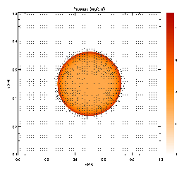
When the control panel settings are to your satisfaction, click the `Plot' button to generate the plot. For Postscript and GIF output, a file is created in the current directory. The result should look something like Figure 3, although this figure was generated from a run with eight levels of refinement rather than the four used in the quick start example run. With fewer levels of refinement the Cartesian grid causes the explosion to appear somewhat diamond-shaped.

FLASH is intended to be customized by the user to work with interesting initial and boundary conditions. In the following sections we will cover in more detail the algorithms and structure of FLASH and the sample problems and tools distributed with it.

3  Algorithmic overview

FLASH provides a general simulation framework capable of incorporating several different types of physics module (e.g., hydrodynamics on structured or unstructured meshes, N-body solvers, reactive source terms, etc.) and initial or boundary conditions. However, it has been built to solve a particular class of problems, namely reactive, compressible flows in astrophysical environments. Thus, FLASH 1.x is distributed with a particular set of algorithms to handle compressible hydrodynamics on a block-structured adaptive mesh, together with an appropriate nuclear equation of state and nuclear reaction network. We treat each of these elements in turn.

3.1  Hydrodynamics

The hydrodynamic module in FLASH 1.x is based on the PROMETHEUS code (Fryxell, Müller, and Arnett 1989). This code solves Euler's equations for compressible gas dynamics in one, two, or three spatial dimensions. These equations can be written in conservative form as

¶r ¶t + Ñ ·rv = 0 (1) ¶rv ¶t + Ñ ·rv v +Ñ P = rg (2) ¶rE ¶t +Ñ ·( rE + P ) v = rv ·g (3)

where r is the fluid density, v is the fluid velocity, P is the pressure, E is the sum of the internal energy e and kinetic energy per unit mass,

E = e+ 1 2 v2 ,

(4)

g is the acceleration due to gravity, and t is the time coordinate. The pressure is obtained from the energy and density using the equation of state. For the case of an ideal gas equation of state, the pressure is given by

P = (g- 1) re,

(5)

where g is the ratio of specific heats. More general equations of state are discussed below.

For reactive flows, a separate advection equation must be solved for each chemical or nuclear species:

¶rXl ¶t + Ñ ·rXl v = 0 ,

(6)

where X_l is the mass fraction of the lth species, with the constraint that å_l X_l = 1. The quantity rX_l represents the partial density of the lth fluid. The code does not explicitly track interfaces between the fluids, so a small amount of numerical mixing can be expected during the course of a calculation.

The equations are solved using a modified version of the Piecewise-Parabolic Method (PPM), which is described in detail in Woodward and Colella (1984) and Colella and Woodward (1984). PPM is a higher-order version of the method developed by Godunov (1959). Godunov's method uses a finite-volume spatial discretization of the Euler equations together with an explicit forward time difference. Time-advanced fluxes at cell boundaries are computed using the analytic solution to Riemann's shock tube problem at each boundary. Initial conditions for each Riemann problem are determined by assuming the nonadvanced solution to be piecewise constant in each cell. Using the Riemann solution has the effect of introducing explicit nonlinearity into the difference equations and permits the calculation of sharp shock fronts and contact discontinuities without introducing significant nonphysical oscillations into the flow. Since the value of each variable in each cell is assumed to be constant, Godunov's method is limited to first-order accuracy in both space and time.

PPM improves on Godunov's method by representing the flow variables with piecewise parabolic functions. It also uses a monotonicity constraint rather than artificial viscosity to control oscillations near discontinuities, a feature shared with the MUSCL scheme of van Leer (1979). Although this could lead to a method which is accurate to third order, PPM is formally accurate only to second order in both space and time, as a fully third-order scheme proved not to be cost-effective. Nevertheless, PPM is considerably more accurate and efficient than most formally second-order algorithms.

PPM is particularly well-suited to flows involving discontinuities, such as shocks and contact discontinuities. The method also performs extremely well for smooth flows, although other schemes which do not perform the extra work necessary for the treatment of discontinuities might be more efficient in these cases. The high resolution and accuracy of PPM are obtained by the explicit nonlinearity of the scheme and through the use of intelligent dissipation algorithms, such as monotonicity enforcement, contact steepening, and interpolant flattening. These algorithms are described in detail by Colella and Woodward (1984).

A complete description of PPM is beyond the scope of this user's guide. However, for comparison with other codes, we note that the implementation of PPM in FLASH 1.x uses the direct Eulerian formulation of PPM and the technique for allowing nonideal equations of state described by Colella and Glaz (1985). For multidimensional problems, FLASH 1.x uses second-order operator splitting (Strang 1968). FLASH also implements PPM on a block-structured adaptive mesh, which is described in the following section.

3.2  Adaptive mesh refinement

We have used a package known as PARAMESH (MacNeice et al. 1999) for the parallelization and adaptive mesh refinement (AMR) portion of FLASH. PARAMESH consists of a suite of subroutines which handle refinement/derefinement, distribution of work to processors, guard cell filling, and flux conservation. In this section we briefly describe this package and the ways in which it has been modified for use with FLASH.

PARAMESH uses a block-structured adaptive mesh refinement scheme similar to others in the literature (e.g., Parashar 1999; Berger & Oliger 1984; Berger & Colella 1989; DeZeeuw & Powell 1993) as well as to schemes which refine on an individual cell basis (Khokhlov 1997). In block-structured AMR, the fundamental data structure is a block of uniform cells arranged in a logically Cartesian fashion. Each cell can be specified using a block identifier (processor number and local block number) and a coordinate triple (i,j,k), where i=1¼nxb, j=1¼nyb, and k=1¼nzb. The complete computational grid consists of a collection of blocks with different physical cell sizes, related to each other in a hierarchical fashion using a tree data structure. The blocks at the root of the tree have the largest cells, while their children have smaller cells and are said to be refined. Two rules govern the establishment of refined child blocks in PARAMESH. First, the cells of a refined child block must be one-half as large as those of its parent block. Second, a block's children must be nested; that is, the child blocks must fit within their parent block and cannot overlap one another, and the complete set of children of a block must fill its volume. Thus, in d dimensions a given block has either zero or 2^d children.

Each block contains nxb×nyb×nzb interior cells and a set of guard cells. The guard cells contain boundary information needed to update the interior cells. These can be obtained from physically neighboring blocks, externally specified boundary conditions, or both. The number of guard cells needed depends upon the interpolation scheme and differencing stencil used for the hydrodynamics algorithm; for the explicit PPM algorithm distributed with FLASH, four guard cells are needed in each direction. PARAMESH handles the filling of guard cells with information from other blocks or a user-specified external boundary routine. If a block's neighbor has the same level of refinement, PARAMESH fills its guard cells using a direct copy from the neighbor's interior cells. If the neighbor has a different level of refinement, the neighbor's interior cells are used to interpolate guard cell values for the block. If the block and its neighbor are stored in the memory of different processors, PARAMESH handles the appropriate parallel communication (blocks are not split between processors). PARAMESH supports only linear interpolation for guard cell filling at jumps at refinement, but it is easily extended to allow other interpolation schemes; for example, for FLASH we have added a quadratic interpolation scheme. Once each block's guard cells are filled, it can be updated independently of the other blocks.

PARAMESH also enforces flux conservation at jumps in refinement, as described by Berger and Colella (1989). At jumps in refinement, the fluxes of mass, momentum, energy, and nuclear abundances across boundary cell faces are averaged across the fine cells at that face and provided to the corresponding coarse face on the neighboring block. These averaged fluxes are then used to update the values of the coarse block's local flow variables.

Each processor decides when to refine or derefine its blocks by computing a user-defined error estimator for each block. Refinement involves creation of between one and 2^d refined child blocks, while derefinement involves deletion of a block. As child blocks are created, they are temporarily placed at the end of the processor's block list. After the refinements and derefinements are complete, the blocks are redistributed among the processors using a work-weighted Morton space-filling curve in a manner similar to that described by Warren and Salmon (1987) for a parallel treecode. During the distribution step each block is assigned a work value (an estimate of the relative amount of time required to update the block). The Morton number of the block is then computed by interleaving the bits of its integer coordinates as described by Warren and Salmon (1987); this determines its location along the space-filling curve. Finally, the list of all blocks is partitioned among the processors using the block weights, equalizing the estimated workload of each processor. During the sorting step, only Morton numbers and not block data are communicated between processors; blocks are only moved (if necessary) after the sort. Changes in refinement are typically performed every ten timesteps.

The refinement criterion used by PARAMESH is adapted from Löhner (1987). Löhner's error estimator was originally developed for finite element applications and has the advantage that it uses an entirely local calculation. Furthermore, the estimator is dimensionless and can be applied with complete generality to any of the field variables of the simulation or any combination of them (by default, PARAMESH uses the density and pressure). Löhner's estimator is a modified second derivative, normalized by the average of the gradient over one computational cell. In one dimension on a uniform mesh it is given by

Ei = | ui+1 - 2ui + ui-1 | | ui+1 - ui | + | ui - ui-1 | + e[ | ui+1 | - 2 | ui | + | ui-1 | ]  ,

(7)

where u_i is the refinement test variable's value in the ith cell. The last term in the denominator of this expression acts as a filter, preventing refinement of small ripples. The constant e is given a value of 10^-4. Although PPM is formally second-order and its leading error terms scale as the third derivative, we have found the second derivative criterion to be very good at detecting discontinuities in the flow variable u. When extending this criterion to multidimensions, all cross derivatives are computed, and the following generalization of the above expresion is used:

Ei = é ê ê ê ê ê ê ê ê ë å k,l  æ ç è ¶2 u ¶xk ¶xl ö ÷ ø é ê ë ( | ¶u ¶xk | i+1 + | ¶u ¶xk | i)/Dxl + e | ¶2 u ¶xk ¶xl | ù ú û 2   ù ú ú ú ú ú ú ú ú û 1/2    ,

(8)

where the sums are carried out over the coordinate directions. If the maximum value of E_i in a block is larger than an adjustable constant, CTORE, the block is marked for refinement. If the maximum value of E_i is less than a second constant (CTODE), the block is marked for derefinement. PARAMESH uses the default values CTORE = 0.8 and CTODE = 0.2. For each block, the error estimator is calculated for all interior cells plus two layers of guard cells, helping to ensure that blocks refine in advance of discontinuities.

3.3  Equation of state

It is common to call an equation of state routine more than 10⁹ times when calculating two- and three-dimensional hydrodynamic models of stellar phenomena. Thus, it is very desirable to have an equation of state that is as efficient as possible, yet accurately represents the relevant physics. While FLASH is easily capable of including any equation of state, here we discuss three equation of state (henceforth EOS) routines which are supplied with FLASH 1.x: the ideal-gas or gamma-law EOS, the Nadyozhin EOS, and the Helmholtz EOS. (The Nadyozhin EOS is no longer supplied with FLASH versions 1.6 and later.)

Each EOS routine takes as input the temperature T, density r, mean number of nucleons per isotope [`A], and mean charge per isotope [`Z]. Each routine then returns as output the scalar pressure (P_tot, specific thermal energy e_tot, and entropy S_tot. In addition to these quantities, the EOS routines return partial derivatives of the pressure, specific thermal energy, and entropy with respect to the density and temperature:

¶Ptot ¶T ê ê ê r   ,       ¶Ptot ¶r ê ê ê T   ,       ¶etot ¶T ê ê ê r   ,       ¶etot ¶r ê ê ê T   ,       ¶Stot ¶T ê ê ê r   ,       ¶Stot ¶r ê ê ê T   .

(9)

Quantities such as the specific heats and the adiabatic indices can be determined once these partial derivatives are known. When solving the energy equation, the temperature usually is obtained by iteration, and the thermodynamic derivatives must be available in order to implement efficient iteration schemes. Confirming that an EOS routine numerically satisfies thermodynamic consistency also demands that the derivatives be available.

An EOS is thermodynamically consistent if its outputs satisfy the Maxwell relations:

P   =  r2   ¶e ¶r ê ê ê T    +  T   ¶P ¶T ê ê ê r  (10) ¶e ¶T ê ê ê r    =   T   ¶S ¶T ê ê ê r  (11) - ¶S ¶r ê ê ê T    =   1 r2   ¶P ¶T ê ê ê r   . (12)

Thermodynamic inconsistency can manifest itself in the unphysical buildup (or decay) of the entropy (or temperature) during numerical simulations of what should be an adiabatic flow. Entropy-sensitive models (e.g., core-collapse supernovae) may suffer inaccuracies if thermodynamic consistency is significantly violated over sufficiently long time scales. The equations of state supplied with FLASH satisfy the Maxwell relations to a good degree of precision (in some cases to the limits of 64-bit arithmetic).

The gamma-law EOS provided with FLASH represents a simple ideal gas with constant adiabatic index g:

P = Na  k _ A rT          e = 1 g- 1   P r           S = P/r+ e T  ,

(13)

where N_a is the Avogadro number, and k is the Boltzmann constant. Because it requires no iteration in order to obtain the temperature, this EOS is quite inexpensive to evaluate.

More complex equations of state are necessary for realistic models of X-ray bursts, Type Ia supernovae, classical novae, and other stellar phenomena, where the electrons and positrons may be relativistic and/or degenerate and where radiation contributes significantly to the thermodynamic state. The Nadyozhin and Helmholtz EOS routines address this need. The Nadyozhin EOS, summarized by Nadyozhin (1974) and explained in detail by Blinnikov et al. (1996), was found by Timmes and Arnett (1999) in a comparison of five different analytic EOS schemes to give the best tradeoff among accuracy, thermodynamic consistency, and speed. The Helmholtz EOS (Timmes & Swesty 1999) uses interpolation from a two-dimensional table of the Helmholtz free energy F(r,T), obtaining comparable accuracy, better thermodynamic consistency, and about twice the speed of the Nadyozhin EOS.

For stellar phenomena, the pressure, specific thermal energy, and entropy contain contributions from several components:

Ptot = Prad + Pion + Pele + Ppos (14) etot = erad + eion +eele + epos (15) Stot = Srad + Sion + Sele + Spos . (16)

Here the subscripts ``rad,'' ``ion,'' ``ele,'' and ``pos'' represent radiation, nuclei, electrons, and positrons, respectively. The radiation portion is that of a blackbody in local thermodynamic equilibrium:

Prad = a T4 3                     erad = 3 Prad r                     Srad = (P/r+ e) T

(17)

where a is the Stefan-Boltzmann energy constant, and c is the speed of light. The ion contribution is that of an ideal gas with g = 5/3. The electrons and positrons are treated as a non-interacting Fermi gas; the number densities of free electrons N_ele and positrons N_pos are given by

Nele = 8 pÖ2 h3   me3  c3  b3/2   [ F1/2(h,b)  +  F3/2(h,b) ] (18) Npos = 8 pÖ2 h3   me3  c3  b3/2 [ F1/2 ( -h- 2/b, b)  +  b  F3/2 ( -h- 2 /b, b) ] , (19)

where h is the Planck constant, m_e is the electron rest mass, b = k T / (m_e c²) is the relativity parameter, h = m/ k T is the normalized chemical potential energy m for electrons, and F_k(h,b) is the Fermi-Dirac integral

Fk(h,b) = ¥ ó õ 0    xk  (1 + 0.5  b x)1/2  dx exp(x - h) + 1  .

(20)

Because the electron rest mass is not included in the chemical potential, the positron chemical potential must have the form h_pos = -h-2/b. For complete ionization, the number density of free electrons in the matter is

Nele,matter = _ Z _ A  Na  r = _ Z    Nion ,

(21)

and charge neutrality requires

Nele,matter = Nele - Npos .

(22)

Solving this equation with a standard one-dimensional root-finding algorithm determines h. Once h is known, the Fermi-Dirac integrals can be evaluated, giving the pressure, specific thermal energy, and entropy due to the free electrons and positrons.

The Nadyozhin EOS routine uses polynomial or rational functions to evaluate the thermodynamic quantities. The temperature-density plane is decomposed into 5 regions (see Figure 12 of Blinnikov et al. 1996), with different expansions or fitting functions applied to each region. The methods used in the 5 regions are (1) a perfect gas approximation with the first-order corrections for degeneracy, (2) expansions of the half-integer Fermi-Dirac functions, (3) Chandrasekhar's (1939) expansion for a degenerate gas, (4) relativistic asymptotics, and (5) Gaussian quadrature for the thermodynamic quantities. The perturbation expansions, asymptotic relations, and fitting functions for the 5 regions are combined, with extraordinary care given to making sure that transitions between the regions are continuous, smooth, and thermodynamically consistent. All of the partial derivatives are obtained analytically.

The electron-positron Helmholtz free energy table used by the Helmholtz EOS was generated by using the Timmes EOS routine (Timmes & Arnett 1999). The Fermi-Dirac integrals, along with their derivatives with respect to h and b, were calculated to at least 18 significant figures using the quadrature schemes of Aparicio (1998). Newton-Raphson iteration was used to solve for h to at least 15 significant figures. The thermodynamic derivatives were computed analytically. Searches through the free energy table are avoided by computing hash indices from the values of any given (T,r[`Z]/[`A]) pair. No computationally expensive divisions are required in interpolating from the table; all of them can be computed and stored the first time the EOS routine is called.

3.4  Thermonuclear reactions

Modelling thermonuclear flashes typically requires the energy generation rate due to nuclear burning over a large range of temperatures, densities and compositions. The average energy generated or lost over a period of time is found by integrating a system of ordinary differential equations (the nuclear reaction network) for the abundances of important nuclei and the total energy release. In some contexts, such as Type II supernova models, the abundances themselves are also of interest. In either case, the coefficients that appear in the equations typically are extremely sensitive to temperature. The resulting stiffness of the system of equations requires the use of an implicit time integration scheme.

Timmes (1999) has reviewed several methods for solving stiff nuclear reaction networks, providing the basis for the reaction network solver included with FLASH. The scaling properties and behavior of three semi-implicit time integration algorithms (a traditional first-order accurate Euler method, a fourth-order accurate Kaps-Rentrop method, and a variable order Bader-Deuflhard method) and eight linear algebra packages (LAPACK, LUDCMP, LEQS, GIFT, MA28, UMFPACK, and Y12M) were investigated by running each of these 24 combinations on seven different nuclear reaction networks (hard-wired 13- and 19-isotope networks and table-lookup networks using 47, 76, 127, 200, and 489 isotopes). Timmes' analysis suggested that the best balance of accuracy, overall efficiency, memory footprint, and ease-of-use was provided by the choice of a 13- or 19-isotope reaction network, the variable order Bader-Deuflhard time integration method, and the MA28 sparse matrix package. The default FLASH distribution uses this combination of methods, which we describe in this section.

We begin by describing the equations solved by the nuclear burning module. We consider material which may be described by a density r and a single temperature T and contains a number of isotopes i, each of which has Z_i protons and A_i nucleons (protons + neutrons). Let n_i and r_i denote the number and mass density, respectively, of the ith isotope, and let X_i denote its mass fraction, so that

Xi = ri/r = ni Ai/(rNA) ,

(23)

where N_A is the Avogadro number. Let the molar abundance of the ith isotope be

Yi = Xi/Ai = ni/(rNA) .

(24)

Mass conservation is then expressed by

N å i=1  Xi = 1

(25)

At the end of each timestep, FLASH checks that the stored abundances satisfy equation (25) to machine precision in order to avoid the unphysical buildup (or decay) of the abundances or energy generation rate. Roundoff errors in this equation can lead to significant problems in some contexts (e.g., classical nova envelopes) where trace abundances are important.

The general continuity equation for the ith isotope is given in Lagrangian formulation by

dYi dt + Ñ·( Yi Vi ) = . Ri    .

(26)

In this equation [(R_i)\dot] is the total reaction rate due to all binary reactions of the form i(j,k)l,

. Ri   = å j,k  Yl Yk lkj(l) - Yi Yj ljk(i) ,

(27)

where l_kj and l_jk are the reverse (creation) and forward (destruction) nuclear reaction rates, respectively. Contributions from three-body reactions, such as the triple-a reaction, are easy to append to equation (27). The mass diffusion velocities V_i in equation (26) are obtained from the solution of a multicomponent diffusion equation (Chapman & Cowling 1970; Burgers 1969; Williams 1988) and reflect the fact that mass diffusion processes arise from pressure, temperature, and/or abundance gradients as well as external gravitational or electrical forces.

The case V_i º 0 is important for two reasons. First, mass diffusion is often unimportant when compared to other transport process such as thermal or viscous diffusion (i.e., large Lewis numbers and/or small Prandtl numbers). Such a situation obtains, for example, in the study of laminar flame fronts propagating through the quiescent interior of a white dwarf. Second, this case permits the decoupling of the reaction network solver from the hydrodynamical solver through the use of operator splitting, greatly simplifying the algorithm. This is the method used by the default FLASH distribution. Setting V_i º 0 transforms equation (26) into

dYi dt = . Ri    ,

(28)

which may be written in the more compact and standard form

. y   = f  (y) .

(29)

Stated another way, in the absence of mass diffusion or advection, any changes to the fluid composition are due to local processes.

Because of the highly nonlinear temperature dependence of the nuclear reaction rates, and because the abundances themselves often range over several orders of magnitude in value, the values of the coefficients which appear in equations (28) and (29) can vary quite significantly. As a result, the nuclear reaction network equations are ``stiff.'' A system of equations is stiff when the ratio of the maximum to the minimum eigenvalue of the Jacobian matrix [(J)\tilde] º ¶f/¶y is large and imaginary. This means that at least one of the isotopic abundances changes on a much shorter timescale than another. Implicit or semi-implicit time integration methods are generally necessary to avoid following this short-timescale behavior, requiring the calculation of the Jacobian matrix.

It is instructive at this point to look at an example of how equation (28) and the associated Jacobian matrix are formed. Consider the ¹²C(a,g)¹⁶O reaction, which competes with the triple-a reaction during helium burning in stars. The rate R at which this reaction proceeds is critical for evolutionary models of massive stars since it determines how much of the core is carbon and how much of the core is oxygen after the initial helium fuel is exhausted. This reaction sequence contributes to the right-hand side equation (29) through the terms

. Y   (4He) = - Y(4He)  Y(12C)  R + ¼ . Y   (12C) = - Y(4He)  Y(12C)  R  + ¼  , (30) . Y   (16O) = + Y(4He)  Y(12C)  R  + ¼

where the ellipsis indicate additional terms coming from other reaction sequences. The minus signs indicate that helium and carbon are being destroyed, while the plus sign indicates that oxygen is being created. Each of these three expressions contributes two terms to the Jacobian matrix [(J)\tilde]=¶f/¶y:

J(4He,4He) = - Y(12C)  R  + ¼           J(4He,12C) = - Y(4He)  R  + ¼ J(12C,4He) = - Y(12C)  R  + ¼           J(12C,12C) = - Y(4He)  R  + ¼  . (31) J(16O,4He) = + Y(12C)  R  + ¼           J(16O,12C) = + Y(4He)  R  + ¼

Entries in the Jacobian matrix represent the flow, in number of nuclei s^-1, into (positive) or out of (negative) an isotope. All of the temperature and density dependence is included in the reaction rate R. The Jacobian matrices that arise from nuclear reaction networks are neither positive-definite nor symmetric since the forward and reverse reaction rates are generally not equal. However, the magnitudes of the matrix entries change as the abundances, temperature, or density change with time.

The default FLASH distribution includes two reaction networks. The 13-isotope a-chain plus heavy-ion reaction network is suitable for most multi-dimensional simulations of stellar phenomena where having a reasonably accurate energy generation rate is of primary concern. The 19-isotope reaction network has the same a-chain and heavy-ion reactions as the 13-isotope network, but it includes additional isotopes to accommodate some types of hydrogen burning (PP and CNO chains), along with some aspects of photodisintegration into ⁵⁴Fe. This reaction network is described in Weaver, Zimmerman, & Woosley (1978). Both the networks supplied with FLASH are examples of ``hard-wired'' reaction networks, where each of the reaction sequences are carefully entered by hand. This approach is suitable for small networks when minimizing the CPU time required to run the reaction network is a primary concern, although it suffers the disadvantage of inflexibility.

The Jacobian matrices of nuclear reaction networks tend to be sparse, and they become more sparse as the number of isotopes increases. Implicit time integration schemes require the inverse of the Jacobian matrix, so we need to use a sparse linear algebra package to compute this inverse. To control the iteration count for a prespecified accuracy, FLASH uses a direct sparse matrix solver. Direct methods typically divide the solution of [(A)\tilde] ·x = b into a symbolic LU decomposition, numerical LU decomposition, and a backsubstitution phase. In the symbolic LU decomposition phase the pivot order of a matrix is determined, and a sequence of decomposition operations which minimize the amount of fill-in is recorded. Fill-in refers to zero matrix elements which become nonzero (e.g., a sparse matrix times a sparse matrix is generally a denser matrix). The matrix is not (usually) decomposed; only the steps to do so are stored. Since the nonzero pattern of a chosen nuclear reaction network does not change, the symbolic LU decomposition is a one-time initialization cost for reaction networks. In the numerical LU decomposition phase, a matrix with the same pivot order and nonzero pattern as a previously factorized matrix is numerically decomposed into its lower-upper form. This phase must be done only once for each staged set of linear equations. In the backsubstitution phase, a set of linear equations is solved with the factors calculated from a previous numerical decomposition. The backsubstitution phase may be performed with as many right-hand sides as needed, and not all of the right-hand sides need to be known in advance.

The MA28 linear algebra package used by FLASH is described by Duff, Erisman, & Reid (1986). It uses a combination of nested dissection and frontal envelope decomposition to minimize fill-in during the factorization stage. An approximate degree update algorithm that is much faster (asymptotically and in practice) than computing the exact degrees is employed. One continuous real parameter sets the amount of searching done to locate the pivot element. When this parameter is set to zero, no searching is done and the diagonal element is the pivot, while when set to unity, complete partial pivoting is done. Since the matrices generated by reaction networks are usually diagonally dominant, the routine is set in FLASH to use the diagonal as the pivot element. Several test cases showed that using partial pivoting did not make a significant accuracy difference, but were less efficient since a search for an appropriate pivot element had to be performed. MA28 accepts the nonzero entries of the matrix in the (i, j, a_i,j) coordinate system, and typically uses uses 70-90% less storage than storing the full dense matrix.

The time integration method used by FLASH for evolving the reaction networks is the variable order Bader-Deuflhard method (e.g., Bader & Deuflhard 1983; Press et al. 1992). The reaction network is advanced over a large time step H from y_n to y_n+1 by the following sequence of matrix equations. First,

h = H/m ( ~ 1   - ~ J   ) ·D0 = h f(yn) (32) y1 = yn + D0 .

Then from k=1,2,¼,m-1

( ~ 1   - ~ J   ) ·x = h f(yk) - Dk-1 Dk = Dk-1 + 2 x (33) yk+1 = yk + Dk  ,

and closure is obtained by the last stage

( ~ 1   - ~ J   ) ·Dm = h [ f (ym) - Dm-1 ] yn+1 = ym + Dm  . (34)

This staged sequence of matrix equations is executed at least twice with m=2 and m=6, yielding a fifth-order method. The sequence may be executed a maximum of seven times, which yields a fifteenth-order method. The exact number of times the staged sequence is executed depends on the accuracy requirements (set to one part in 10⁶ in FLASH) and the smoothness of the solution. Estimates of the accuracy of an integration step are made by comparing the solutions derived from different orders. The minimum cost of this method - which applies for a single time step that met or exceeded the specified integration accuracy - is one Jacobian evaluation, eight evaluations of the right-hand side, two matrix decompositions, and ten backsubstitutions. This minimum cost can be increased at a rate of one decomposition (the expensive part) and m backsubstitutions (the inexpensive part) for every increase in the order 2k+1. The cost of increasing the order is compensated for, hopefully, by taking a correspondingly larger (but accurate) time step. The controls for order versus step size are a built-in part of the Bader-Deuflhard method. The cost per step of this integration method is at least twice as large as the cost per step of either a traditional first-order accurate Euler method or a fourth-order accurate Kaps-Rentrop (essentially an implicit Runge-Kutta) method, However, if the Bader-Deuflhard method can take accurate time steps that are at least twice as large, then this method will be more efficient globally. Timmes (1999) shows that this is typically the case. Note that in equations (32) - (34) not all of the right-hand sides are known in advance since the sequence of linear equations is staged. This staging feature of the integration method will make some matrix packages, such as MA28, a more efficient choice.

The energy generation rate is given by the sum

. e   nuc  = NA   å i    dYi dt  .

(35)

Note that a nuclear reaction network does not need to be evolved in order to obtain the instantaneous energy generation rate, since only the right hand sides of the ordinary differential equations need to be evaluated. It is more appropriate in the FLASH program to use the average nuclear energy generated over a time step

. e   nuc  = NA   å i    DYi Dt  .

(36)

In this case, the nuclear reaction network does need to be evolved. The energy generation rate, after subtraction of any neutrino losses, is returned to the FLASH program for use with the operator splitting technique.

Finally, the tabulation of Caughlan & Fowler (1988) is used in FLASH for most of the key nuclear reaction rates. Modern values for some of the reaction rates were taken from the reaction rate library of Hoffman (1999, priv. comm.). Nuclear reaction rate screening effects as implemented by Wallace, Woosley, & Weaver (1982), and decreases in the energy generation rate [(e)\dot]_nuc due to neutrino losses as given by Itoh et al. (1985) are included in calculations done with FLASH.

4  FLASH tools

In this section we describe several of the tools distributed with FLASH. The source code for these programs (except for setup) can be found in the main FLASH source tree under the tools/ directory.

4.1  The FLASH configuration script (setup)

The setup script, found in the FLASH root directory, provides the primary command-line interface to the FLASH source code. It configures the source tree for a given problem and target machine and creates files needed to parse the runtime parameter file and make the FLASH executable. More description of what setup does may be found in Section 6.1. Here we describe its basic usage.

Running setup without any options prints a message describing the available options:

[sphere 5:09pm] % ./setup
usage: setup <problem-name> [options]

              problems: see ./setups
              options: -verbose -portable -defaults -[123]d -maxblocks=<#>
                           [-site=<site> | -ostype=<ostype>]

For compatibility with older versions of setup, the syntax
              setup <problem-name> <ostype> [options]
is also accepted, so long as <ostype> does not begin with a dash (-).
In this case the -site and -ostype options cannot be used.

A ``problem'' consists of a set of initial and boundary conditions, possibly additional physics (e.g., a subgrid model for star formation), and a set of adjustable parameters. The directory associated with a problem contains source code files which implement the initial and boundary conditions and extra physics, together with a configuration file, read by setup, which contains information on required physics modules and adjustable parameters.

setup determines site-dependent configuration information by looking in source/sites/ for a directory with the same name as the output of the hostname command; failing this, it looks in source/sites/Prototypes/ for a directory with the same name as the output of the uname command. The site and operating system type can be overridden with the -site and -ostype command-line options. Only one of these options can be used. The directory for each site or operating system type contains a makefile fragment ( Makefile.h) that sets command names, compiler flags, and library paths, and any replacement or additional source files needed to compile FLASH for that machine type.

setup uses the problem and site/OS type, together with a user-supplied file called Modules which lists the code modules to include, to generate a directory called object/ which contains links to the appropriate source files and makefile fragments. It also creates the master makefile (object/Makefile) and several Fortran include files that are needed by the code in order to parse the runtime parameter file. After running setup, the user can make the FLASH executable by running gmake in the object/ directory (or from the FLASH root directory, if the -portable option is not used with setup). The optional command-line modifiers have the following interpretations:

# Modules file constructed for rt problem by setup -defaults INCLUDE driver/time_dep INCLUDE hydro INCLUDE materials/eos/gamma INCLUDE gravity/constant INCLUDE mesh INCLUDE io

After configuring the source tree with setup and using gmake to create an executable in the build directory, look in the build directory for a file named rt_parms.txt. This contains a complete list of all of the runtime parameters available to the executable, together with their variable types, default values, and comments. To set runtime parameters to values other than the defaults, create a runtime parameter file named flash.par in the directory from which FLASH is to be run. The format of this file is described in Section 2.

4.2  FLASH output comparison utility (focu)

The FLASH output comparison utility, or focu (pronounced faux-coup), is a command-line utility which compares FLASH output files according to specified criteria (e.g., local or global error criterion on any of the hydrodynamical variables) and reports whether they are the same or not. This is useful in determining whether a change to FLASH (or to the value of a runtime parameter) has changed the results obtained with a given problem.

4.2.1  Building focu

The focu executable is configured and built in much the same way as is FLASH: obtain source tree, run setup to configure the source tree for a given architecture, and run gmake in the build directory. FLASH and focu are different in that focu is problem-independent, so only a machine type needs to be specified, and in that (at least at the present time) all of the modules included with focu are used, so setup is always run with the -defaults option. (See Section 4.1 for details regarding the usage of setup.) To summarize the steps in building focu:

1. Move to the focu root directory (tools/focu/ relative to the FLASH root directory).
2. Run ./setup -defaults. As with the FLASH setup script, the -site and -ostype options can be used to specify a site configuration or operating system prototype. Do not use the setup script in the FLASH root directory.
3. Edit object/Makefile.h to set compiler flags and the locations of libraries. Since focu contains routines to read HDF 4 output, you must have the HDF 4 library installed.
4. Run gmake. If compilation is successful, you should find an executable named focu in the current directory.

4.2.2  Using focu

Running focu is very similar to running FLASH itself. First prepare a runtime parameter file, then run focu using

mpirun -np N focu parameter-file

The runtime parameters understood by focu are as follows. Default values are listed in brackets following each description.

FOCU: Flash Output Comparison Utility Comparing: sedov_4_hdf_chk_0003 ( 69 blocks) sedov_4_hdf_chk_0003 ( 69 blocks) Variable: density Criterion: local sum Threshold: 1.0000000000000E-09 Result:   Error: 0.0000000000000E+00   Minimum: 0.0000000000000E+00   Maximum: 0.0000000000000E+00   SUCCESS

The output of focu is a short report listing the volume-averaged sum, minimum, and maximum deviations (local or global, depending on the setting of criterion) and reporting SUCCESS or FAILURE according to the supplied threshold. An example report generated by focu is shown in Figure 5. Note that the last line of the report begins with SUCCESS or FAILURE, making it easy for a script to test the results. For example, with csh one might use

set result = `mpirun -np 2 focu focu_sedov.par | grep SUCCESS`
if ("result" == "SUCCESS") then
...
endif

focu is used by the automated FLASH test script (Section 5.1) to compare FLASH outputs to the reference results supplied as part of the test suite.

4.3  IDL routines for the analysis of FLASH output (fidlr)

fidlr is a set of routines, written in the IDL language, that can plot or read data files produced by FLASH. The routines include programs which can be run from the IDL command line to read 1D, 2D, or 3D FLASH datasets and interpolate them onto uniform grids. Other IDL programs (xflash and cousins) provide a graphical interface to these routines, enabling users to read and plot AMR datasets without interpolating onto a uniform mesh.

Currently, the fidlr routines support 1, 2, and 3-dimensional datasets in the FLASH HDF 4 or HDF 5 formats. Both plotfiles and checkpoint files are supported, as they differ only in the number of variables stored, and possibly the numerical precision. Since IDL does not directly support HDF 5, the call_external function is used to interface with a set of C routines that read in the HDF 5 data. Using these routines requires that the HDF 5 library be installed on your system and that the shared-object library be compiled before reading in data. Since the call_external function is used, the demo version of IDL will not run the routines.

For basic plotting operations, the easiest way to generate plots of FLASH data is to use one of the widget interfaces: xflash for 2d data, xflash1d for 1d data, and xflash3d for 3d data. For more advanced analysis, the read routines can be used to read the data into IDL, and it can then be accessed through the common blocks. Examples of using the fidlr routines from the command line are provided in Section 4.3.5. Additionally, some scripts demonstrating how to analyze FLASH data using the fidlr routines are described in Section 4.3.5 (see for example radial.pro).

The driver routines provided with fidlr visualize the AMR data by first converting it to a uniform mesh. This allows for ease of plotting and manipulation, but it is less efficient than plotting the native AMR structure. Analysis can still be performed directly on the native data through the command line.

4.3.1  Installing and running fidlr

fidlr is distributed with FLASH and contained in the tools/fidlr/ directory. In addition to the IDL procedures, a README file is present which will contain up-to-date information on changes and installation requirements.

These routines were written and tested using IDL v5.3 for IRIX. They should work without difficulty on any UNIX machine with IDL installed. Any functionality of fidlr under Windows is purely coincidental. Later versions of IDL are rumored to no longer support GIF files due to copyright difficulties, so outputting to a image file may not work. It is possible to run IDL in a `demo' mode if there are not enough licenses available. Unfortunately, some parts of fidlr will not function in this mode, as certain features of IDL are disabled. This guide assumes that you are running the full version of IDL.

Installation of fidlr requires defining some environment variables, and compiling the support for HDF 5 files. These procedures are described below.

Setting up fidlr environment variables

The FLASH IDL routines are located in the tools/fidlr/ subdirectory of the FLASH root directory. To use them you must set two environment variables. First set the value of XFLASH_DIR to the location of the FLASH IDL routines; for example, under csh, use

setenv XFLASH_DIR flash-root-path/tools/fidlr

Next add this directory to your IDL_PATH variable:

setenv IDL_PATH "${XFLASH_DIR}:$IDL_PATH"

Setting up the HDF 5 routines

For fidlr to read HDF 5 files, you need to install the HDF 5 library on your machine and compile the wrapper routines. The HDF 5 libraries can be obtained in either source or binary form for most Unix platforms from http://hdf.ncsa.uiuc.edu. The Makefile supplied will create the shared-object library on an SGI, but will need to be edited for other platforms. The compiler flags for a shared-object library for different versions of Unix can be found in

$IDL_DIR/external/call_external/C/callext_unix.txt

It is important that you compile the shared-object to conform to the same application binary interface (ABI) that IDL was compiled with. On an SGI, IDL version 5.2.1 and later use the n32 ABI, while versions before this are o32. The HDF library will also need to be compiled in the same format.

IDL interacts with external programs through the call_external function. Any arguments are passed by reference through argc and argv. These are recast into pointers of the proper type in the C routines. The C wrappers call the appropriate HDF functions to read the data and return it through the argc pointers.

Running IDL

fidlr uses 8-bit color tables for all of its plotting. On displays with higher colordepths, it may be necessary to use color overlays to get the proper colors on your display. For SGI machines, launching IDL with the start.pro script with enable 8-bit pseudocolor overlays.

4.3.2  fidlr data structures

The fidlr routines access the data contained in the FLASH output files through a series of common blocks. For the most part, the variable names are consistent with the names used in FLASH. It is assumed that the user is familiar with the block structured AMR format employed by FLASH. All of the unknowns are stored together in the unk data-structure, which mirrors that contained in FLASH itself. The list of variable names is contained in the string array unk_names. A utility function var_index is provided to convert between a 4-character string name and the index into unk. For example,

unk[var_index('dens'),*,*,*,*]

fidlr will attempt to create derived variables from the variables stored in the output file if it can. For example, the total velocity can be created from the components of the velocity, if they are all present. A separate data structure varnames contains the list of variables in the output file plus any additional variables fidlr knows how to derive.

At present, the global common blocks defined by fidlr are:

common size, tot_blocks, nvar, nxb, nyb, nzb, ntopx, ntopy, ntopz
common time, time, dt
common tree, lrefine, nodetype, gid, coord, size, bnd_box
common vars, unk, unk_names

IDL> .run def_common
IDL> read_amr, 'filename_hdf_chk_0000'
IDL> leaf_blocks = where(nodetype EQ 1)
IDL> print, min(unk[var_index('dens'),*,*,*,leaf_blocks])

4.3.3  xflash: plotting two-dimensional datasets

The main interface to the fidlr routines for plotting 2-dimensional data sets is xflash. xflash produces colormap plots of FLASH data with optional velocity vectors, contours, and the AMR block structure overlaid. The basic operation of xflash is to specify a file or range of files, probe the file for the list of variables it contains (through the discover variables button described below), and then specify the remaining plot options.

xflash can output to the screen, postscript, or an image file (GIF). If the data is significantly higher resolution than the output device, then xflash (through xplot_amr.pro) will sub-sample the image by one or more levels of refinement before plotting.

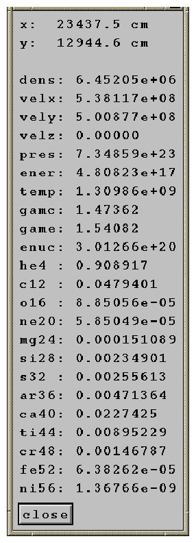
Once the image is plotted, the query button will become active. Pressing query and then clicking anywhere in the domain will pop up a window containing the values of all the FLASH variables in the zone nearest the cursor.

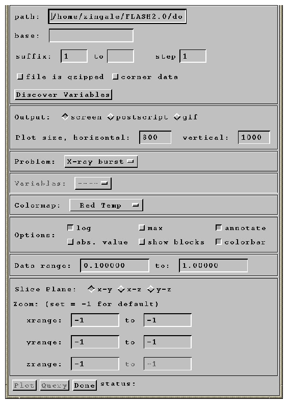
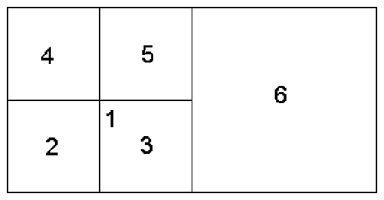
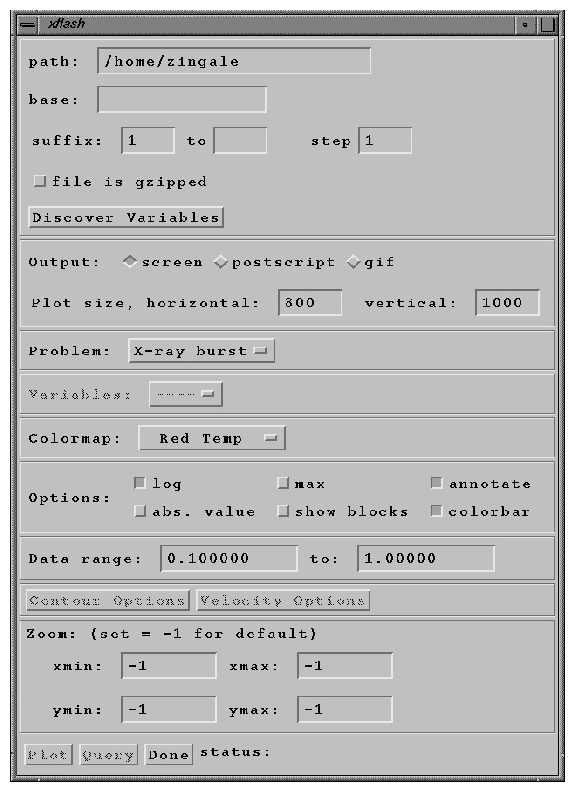
Typing xflash at the IDL command prompt will launch the main xflash widget, shown in Figure 6(a). The widget is broken into several sections, with some features initially disabled. These sections are explained below.

 
File Options

The file to be visualized is composed of the path, the basename (the same base name used in the flash.par) plus any file type information appended to it (ex. 'hdf_chk_') and the range of suffices to loop through. An optional parameter, step, controls how many files to skip when looping over the files. By default, xflash sets the path to the working directory that IDL was started from. xflash will spawn gzip if the file is stored on disk compressed and the file is gzipped box is checked. After the file is read, it will be compressed again.

Once the file options are set, clicking on discover variables will read the variable list from the first file specified, and use the variable names to populate the variable selection box. xflash will automatically determine if the file is an HDF 4 or 5 file, and read the `unknown names' record to get the variable list. This will work for both plotfiles and checkpoint files generated by FLASH.

 
Output Options

A plot can be output to the screen (default), a Postscript file, or a GIF file. The output filenames are composed from the basename + variable name + suffix. For outputs to the screen or GIF, the plot size options allow you to specify the image size in pixels. For Postscript output, xflash chooses portrait or landscape orientation depending on the aspect ratio of the domain.

 
Problem

The problem dropbox allows you to select one of the predefined problem defaults. This will load the options (data ranges, velocity parameters, and contour options) for the problem as specified in the xflash_defaults procedure. When xflash is started, xflash_defaults is executed to read in the known problem names. To add a problem to xflash, only the xflash_defaults procedure needs to be modified. The details of this procedure are provided in the comment header in xflash_defaults. It is not necessary to add a problem in order to plot a dataset, as all default values can be overridden through the widget.

 
Variables

The variables dropbox lists the variables stored in the `unknown names' record in the data file, and any derived variables that xflash knows how to construct from these variables (ex: sound speed). This allows you to choose the variable to be plotted. By default, xflash reads all the variables in a file, so switching the variable to plot can be done without rereading.

 
Colormap

The colormap dropbox lists the available colormaps to xflash. These colormaps are stored in flash_colors.tbl in the fidlr directory, and differ from the standard IDL colormaps. The first 12 colors in the colormaps are reserved by xflash to hold the primary colors used for different aspects of the plotting. Additional colormaps can be created by using the xpalette function in IDL.

 
Options

The options block allows you to toggle various options on/off (Table 3).

 
 
Data Range

These fields allow you to specify the range of the variable to plot. Data outside of the range will be scaled to the minimum and maximum values of the colormap respectively.

 
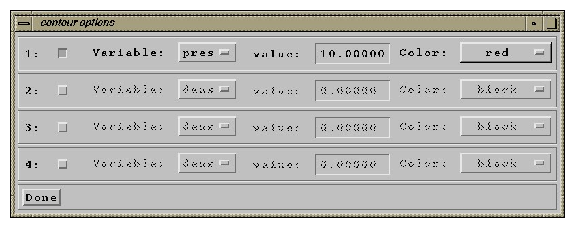
Contour Options

This launches a dialog box that allows you to select up to 4 contour lines to overplot of the data (see figure 7). The variable, value, and color are specified for each reference contour. To plot a contour, select the check box next to the contour number. This will allow you to set the variable to make the contour from, the value of the contour, and the color.

Figure 7: The xflash contour option subwidget.

 
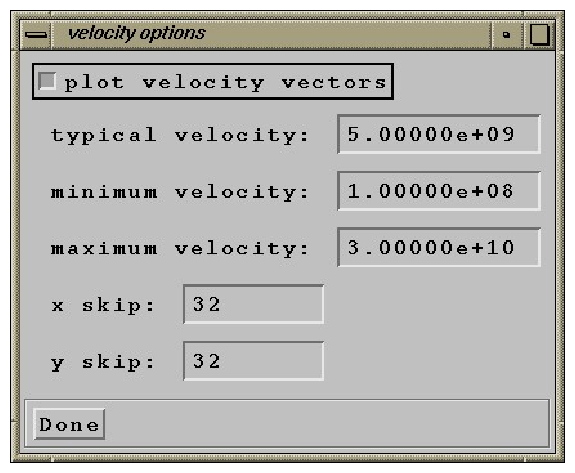
Velocity Options

This launches a dialog box that allows you to set the velocity options used to plot velocity vectors on the plot (see figure 8). The plotting of velocity vectors is controlled by the partvelvec.pro procedure. xskip and yskip allow you to thin out the arrows. typical velocity sets the velocity to scale the vectors to, and minimum velocity and maximum velocity specify the range of velocities to plot vectors for.

Figure 8: The xflash velocity option subwidget.

 
Zoom

The zoom options allow you to set the domain limits for the plot. A value of -1 uses the actual limit of the domain.

 
Plot

Create the plot. The status of the plot will appear on the status bar at the bottom.

 
Query

The query button becomes active once the plot is created. Clicking on query and then clicking somewhere in the domain lists the data values at the cursor location (see Figure 9).

Figure 9: The xflash query widget, displaying information for a zone.

4.3.4  xflash3d: plotting slices of three-dimensional datasets

xflash3d provides an interface for plotting slices of 3-dimension FLASH datasets. It is written to conserve memory-only a single variable is read in at a time, and only the slice to be plotted is put on a uniform grid. The merging of the AMR data to a uniform grid is accomplished by merge3d_amr.pro which can take a variety of arguments which control what volume of the domain is to be put onto a uniform grid.

Figure 10: The xflash3d widget.

Figure 10 shows the main xflash3d widget. The interface is similar to that of xflash, so the above description from that section still applies. The major difference is in the zoom section, which controls the slice plane.

The slice plane button group controls the plane to plot the data in. For a given plane, the direction orthogonal will have only on active text box to enter zoom information-this controls the position of the slice plane in the normal direction. For the directions in the slice plane, the zoom boxes allow you to select a sub-domain in that plane to plot.

4.3.5   The fidlr command-line routines

Table 4 lists all of the fidlr routines, grouped by function. Most of these routines rely on the common blocks to get the tree structure necessary to interpret a FLASH dataset. Command line analysis of FLASH data requires that the common blocks be defined, usually by executing def_common.pro.

IDL command-line example

Most of the fidlr routines can be used directly from the command line to perform analysis not offered by the different widget interfaces. This section provides an example of using the fidlr routines.

 
Example. Generate a contour plot of density from a 3-d dataset in the x-z plane at the y midpoint.

IDL> .run def_common
IDL> read_amr, 'filename_hdf_chk_0000'
IDL> sdens = merge3d_amr(unk[var_index('dens'),*,*,*,*], $
IDL>   xmerge=x, ymerge=y, zmerge=z)
IDL> help, sdens
sdens       FLOATArray[256, 256, 256]
IDL> contour, reform(sdens[*,128,*]), x, z

5  The supplied problems

5.1  Running the FLASH test suite

To verify that FLASH works as expected, and to debug changes in the code, we have created a suite of standard test problems. Most of these problems have analytical solutions which can be used to test the accuracy of the code. The remaining problems do not have analytical solutions, but they produce well-defined flow features which have been verified by experiments and are stringent tests of the code. The test suite configuration code is included with the FLASH source tree (in the setups/ directory), so it is easy to configure and run FLASH with any of these problems `out of the box.' Sample runtime parameter files are also included. Files containing reference results for the test suite tend to be large and so are distributed separately (via the FLASH_TEST CVS tree or in archive form as FLASH_TEST.tar). The FLASH_TEST tree also contains the runtime parameter files needed to reproduce the reference results.

Included with the test suite results is a script named flash_test which automates the process of comparing test suite results with the reference results. flash_test takes one argument, the machine type (run flash_test with no arguments for a list of available types). It automatically configures and builds FLASH for each of the test problems, builds the focu output comparison utility (Section 4.2), runs FLASH with each test problem, and uses focu to compare the results. It prepares a report for the entire suite of problems, flagging compilation problems, catastrophic runtime errors, and erroneous results. Since flash_test can be quite time-consuming to execute for the full test suite, it is generally a good idea to execute it as a batch job on the target system. Note that the tests may be run individually using the runtime parameter files provided with the FLASH test suite. Plots similar to those in this section can be produced using IDL routines provided with the test suite; these make use of the FLASH IDL tools (Section 4.3).

5.2  The Sod shock-tube problem

The Sod problem (Sod 1978) is an essentially one-dimensional flow discontinuity problem which provides a good test of a compressible code's ability to capture shocks and contact discontinuities with a small number of zones and to produce the correct density profile in a rarefaction. It also tests a code's ability to correctly satisfy the Rankine-Hugoniot shock jump conditions. When implemented at an angle to a multidimensional grid, it can also be used to detect irregularities in planar discontinuities produced by grid geometry or operator splitting effects.

We construct the initial conditions for the Sod problem by establishing a planar interface at some angle to the x and y axes. The fluid is initially at rest on either side of the interface, and the density and pressure jumps are chosen so that all three types of flow discontinuity (shock, contact, and rarefaction) develop. To the ``left'' and ``right'' of the interface we have

rL = 1 rR = 0.125 pL = 1 pR = 0.1

(37)

The ratio of specific heats g is chosen to be 1.4 on both sides of the interface.

In FLASH, the Sod problem (sod) uses the runtime parameters listed in Table 5 in addition to the regular ones supplied with the code. For this problem we use the gamma equation of state module and set the value of the parameter gamma supplied by this module to 1.4. The default values listed in Table 5 are appropriate to a shock with normal parallel to the x-axis which initially intersects that axis at x=0.5 (halfway across a box with unit dimensions).

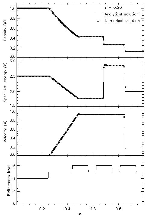
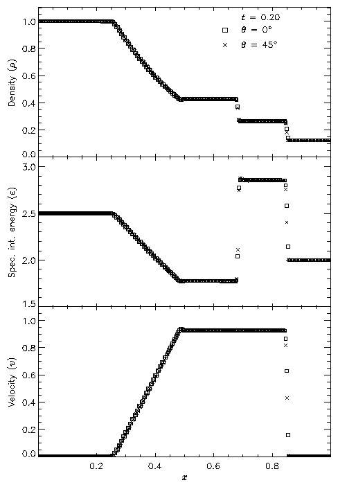
Figure 11 shows the result of running the Sod problem with FLASH on a two-dimensional grid, with the analytical solution shown for comparison. The hydrodynamical algorithm used here is the directionally split piecewise-parabolic method (PPM) included with FLASH. In this run the shock normal is chosen to be parallel to the x-axis. With six levels of refinement, the effective grid size at the finest level is 256², so the finest zones have width 0.00390625. At t=0.2 three different nonlinear waves are present: a rarefaction between x » 0.25 and x » 0.5, a contact discontinuity at x » 0.68, and a shock at x » 0.85. The two sharp discontinuities are each resolved with approximately three zones at the highest level of refinement, demonstrating the ability of PPM to handle sharp flow features well. Near the contact discontinuity and in the rarefaction we find small errors of about 1-2% in the density and specific internal energy, with similar errors in the velocity inside the rarefaction. Elsewhere the numerical solution is exact; no oscillation is present.

Figure 12 shows the result of running the Sod problem on the same two-dimensional grid with different shock normals: parallel to the x-axis (q = 0^°) and along the box diagonal (q = 45^°). For the diagonal solution we have interpolated values of density, specific internal energy, and velocity to a set of 256 points spaced exactly as in the x-axis solution. This comparison shows the effects of the second-order directional splitting used with FLASH on the resolution of shocks. At the right side of the rarefaction and at the contact discontinuity the diagonal solution undergoes slightly larger oscillations (on the order of a few percent) than the x-axis solution. Also, the value of each variable inside the discontinuity regions differs between the two solutions by up to 10% in most cases. However, the location and thickness of the discontinuities is the same between the two solutions. In general shocks at an angle to the grid are resolved with approximately the same number of zones as shocks parallel to a coordinate axis.

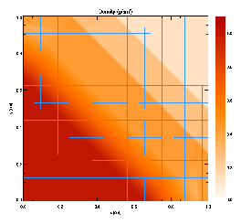
Figure 13 presents a grayscale map of the density at t=0.2 in the diagonal solution together with the block structure of the AMR grid in this case. Note that regions surrounding the discontinuities are maximally refined, while behind the shock and discontinuity the grid has de-refined as the second derivative of the density has decreased in magnitude. Because zero-gradient outflow boundaries were used for this test, some reflections are present at the upper left and lower right corners, but at t=0.2 these have not yet propagated to the center of the grid.

5.3  The Woodward-Colella interacting blast-wave problem

This problem was originally used by Woodward and Colella (1984) to compare the performance of several different hydrodynamical methods on problems involving strong, thin shock structures. It has no analytical solution, but since it is one-dimensional, it is easy to produce a converged solution by running the code with a very large number of zones, permitting an estimate of the self-convergence rate when narrow, interacting discontinuities are present. For FLASH it also provides a good test of the adaptive mesh refinement scheme.

The initial conditions consist of two parallel, planar flow discontinuities. Reflecting boundary conditions are used. The density in the left, middle, and right portions of the grid (r_L, r_M, and r_R, respectively) is unity; everywhere the velocity is zero. The pressure is large to the left and right and small in the center:

pL = 1000 pM = 0.01 pR = 100 .

(38)

The equation of state is that of a perfect gas with g = 1.4.

Figure 14 shows the density and velocity profiles at several different times in the converged solution, demonstrating the complexity inherent in this problem. The initial pressure discontinuities drive shocks into the middle part of the grid; behind them, rarefactions form and propagate toward the outer boundaries, where they are reflected back onto the grid and interact with themselves. By the time the shocks collide at t=0.028, the reflected rarefactions have caught up to them, weakening them and making their post-shock structure more complex. Because the right-hand shock is initially weaker, the rarefaction on that side reflects from the wall later, so the resulting shock structures going into the collision from the left and right are quite different. Behind each shock is a contact discontinuity left over from the initial conditions (at x » 0.50 and 0.73). The shock collision produces an extremely high and narrow density peak; in the Woodward and Colella calculation the peak density is slightly less than 30. Even with ten levels of refinement, FLASH obtains a value of only 18 for this peak. Reflected shocks travel back into the colliding material, leaving a complex series of contact discontinuities and rarefactions between them. A new contact discontinuity has formed at the point of the collision (x » 0.69). By t=0.032 the right-hand reflected shock has met the original right-hand contact discontinuity, producing a strong rarefaction which meets the central contact discontinuity at t=0.034. Between t=0.034 and t=0.038 the slope of the density behind the left-hand shock changes as the shock moves into a region of constant entropy near the left-hand contact discontinuity.

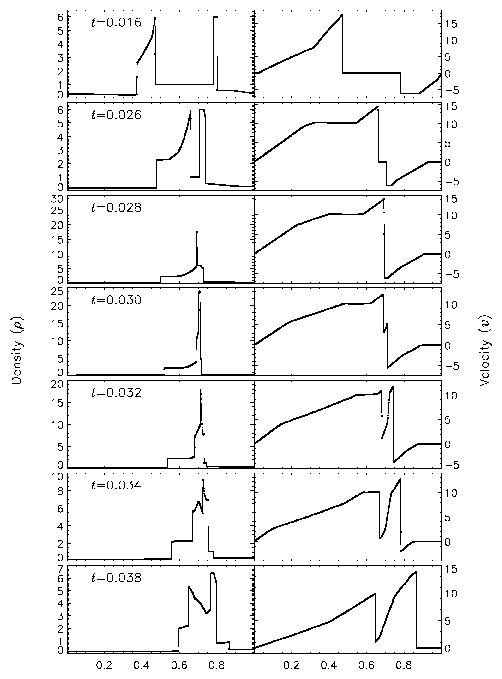
Figure 15 shows the self-convergence of density and pressure when FLASH is run on this problem. For several runs with different maximum refinement levels, we compare the density, pressure, and total specific energy at t=0.038 to the solution obtained using FLASH with ten levels of refinement. This figure plots the L1 error norm for each variable u, defined using

E(Nref;u) º 1 N(Nref) N(Nref) å i=1  ê ê ê ui(Nref) -ui(10) ui(10) ê ê ê  ,

(39)

against the effective number of zones (N(N_ref)) at the highest level of refinement N_ref. In computing this norm, both the `converged' solution u(10) and the test solution u(N_ref) are interpolated onto a uniform mesh having N(N_ref) zones. Values of N_ref between 2 (corresponding to cell size Dx=1/16) and 9 (Dx=1/2048) are shown.

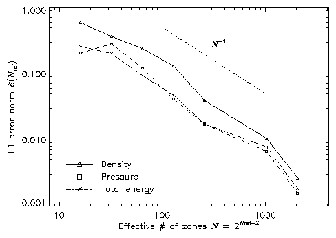
Although PPM is formally a second-order method, one sees from this plot that, for the interacting blast-wave problem, the convergence rate is only linear. Indeed, in their comparison of the performance of seven nominally second-order hydrodynamic methods on this problem, Woodward and Colella found that only PPM achieved even linear convergence; the other methods were worse. The error norm is very sensitive to the correct position and shape of the strong, narrow shocks generated in this problem.

The additional runtime parameters supplied with the 2blast problem are listed in Table 6. This problem is configured to use the perfect-gas equation of state (gamma), and it is run in a two-dimensional unit box with gamma set to 1.4. Boundary conditions in the y direction (transverse to the shock normals) are taken to be periodic.

5.4  The Sedov explosion problem

The Sedov explosion problem (Sedov 1959) is another purely hydrodynamical test in which we check the code's ability to deal with strong shocks and non-planar symmetry. The problem involves the self-similar evolution of a cylindrical or spherical blast wave from a delta-function initial pressure perturbation in an otherwise homogeneous medium. To initialize the code, we deposit a quantity of energy E=1 into a small region of radius dr at the center of the grid. The pressure inside this volume, p₀¢, is given by

p0¢ = 3(g-1)E (n+1)p drn  ,

(40)

where n = 2 for cylindrical geometry and n = 3 for spherical geometry. We set g = 1.4. (In running this problem we choose dr to be 3.5 times as large as the finest adaptive mesh resolution in order to minimize effects due to the Cartesian geometry of our grid.) Everywhere the density is set equal to r₀=1, and everywhere but the center of the grid the pressure is set to a small value, p₀=10^-5. The fluid is initially at rest. In the self-similar blast wave which develops for t > 0, the density, pressure, and radial velocity are all functions of x º r/R(t), where

R(t) = Cn(g) æ ç è Et2 r0 ö ÷ ø 1/(n+2)    .

(41)

Here C_n is a dimensionless constant depending only on n and g; for g = 1.4, C₂ » C₃ » 1 to within a few percent. Just behind the shock front at x = 1 we have

r = r1   º g+1 g-1 r0 p = p1   º 2 g+1 r0 u2 (42) v = v1   º 2 g+1 u ,

where u º dR/dt is the speed of the shock wave. Near the center of the grid,

r(x)/r1 µ xn/(g-1) p(x)/p1 = constant  . (43) v(x)/v1 µ x

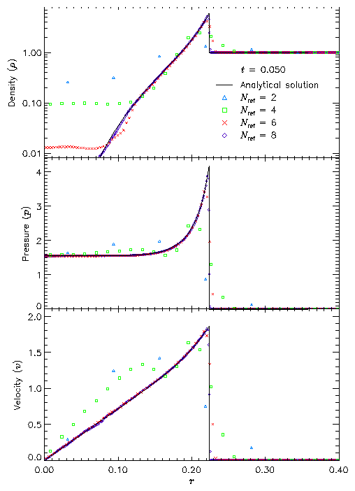
Figure 16 shows density, pressure, and velocity profiles in the two-dimensional Sedov problem at t=0.05. Solutions obtained with FLASH on grids with 2, 4, 6, and 8 levels of refinement are shown in comparison with the analytical solution. In this figure we have computed average radial profiles in the following way. We interpolated solution values from the adaptively gridded mesh used by FLASH onto a uniform mesh having the same resolution as the finest AMR blocks in each run. Then, using radial bins with the same width as the zones in the uniform mesh, we binned the interpolated solution values, computing the average value in each bin. At low resolutions, errors show up as density and velocity overestimates behind the shock, underestimates of each variable within the shock, and a numerical precursor spanning 1-2 zones in front of the shock. However, the central pressure is accurately determined, even for two levels of refinement; because the density goes to a finite value rather than its correct limit of zero, this corresponds to a finite truncation of the temperature (which should go to infinity as r® 0). As resolution improves, the artificial finite density limit decreases; by N_ref=6 it is less than 0.2% of the peak density. Except for the N_ref=2 case, which does not show a well-defined peak in any variable, the shock itself is always captured with about two zones. The region behind the shock containing 90% of the swept-up material is represented by four zones in the N_ref=4 case, 17 zones in the N_ref=6 case, and 69 zones for N_ref=8. However, because the solution is self-similar, for any given maximum refinement level the shock will be four zones wide at a sufficiently early time. The behavior when the shock is underresolved is to underestimate the peak value of each variable, particularly the density and pressure.

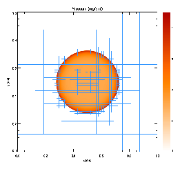
Figure 17 shows the pressure field in the 8-level calculation at t=0.05 together with the block refinement pattern. Note that a relatively small fraction of the grid is maximally refined in this problem. Although the pressure gradient at the center of the grid is small, this region is refined because of the large temperature gradient there. This illustrates the ability of PARAMESH to refine grids using several different variables at once.

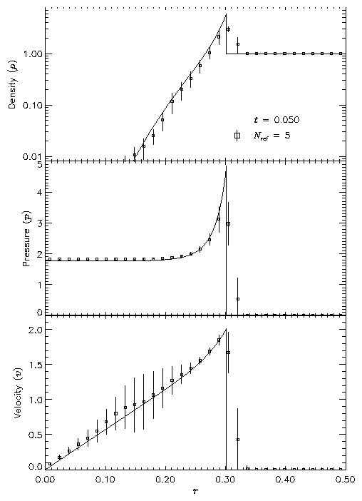
We have also run FLASH on the spherically symmetric Sedov problem in order to verify the code's performance in three dimensions. The results at t=0.05 using five levels of grid refinement are shown in Figure 18. In this figure we have plotted the root-mean-square (RMS) numerical solution values in addition to the average values. As in the two-dimensional runs, the shock is spread over about two zones at the finest AMR resolution in this run. The width of the pressure peak in the analytical solution is about 1 1/2 zones at this time, so the maximum pressure is not captured in the numerical solution. Behind the shock the numerical solution average tracks the analytical solution quite well, although the Cartesian grid geometry produces RMS deviations of up to 40% in the density and velocity in the derefined region well behind the shock. This behavior is similar to that exhibited in the two-dimensional problem at comparable resolution.

The additional runtime parameters supplied with the sedov problem are listed in Table 7. This problem is configured to use the perfect-gas equation of state (gamma), and it is run in a unit box with gamma set to 1.4.

5.5  The advection problem

In this problem we create a planar density pulse in a region of uniform pressure p₀ and velocity u₀, with the velocity normal to the pulse plane. The density pulse is defined via

r(s) = r1f(s/w) + r0[1-f(s/w)] ,

(44)

where s is the distance of a point from the pulse midplane, w is the characteristic width of the pulse, and the pulse shape function f is, for a square pulse,

fSP(x) = ì í î 1     |x| < 1 0     |x| > 1  ,

(45)

and for a Gaussian pulse,

fGP(x) = e-x2 .

(46)

For these initial conditions the Euler equations reduce to a single wave equation with wave speed u₀; hence the density pulse should move across the computational volume at this speed without changing shape. Advection problems similar to this were first proposed by Boris and Book (1973) and Forester (1977).

The advection problem tests the ability of the code to handle planar geometry, as does the Sod problem. It is also like the Sod problem in that it tests the code's treatment of flow discontinuities which move at one of the characteristic speeds of the hydrodynamical equations. (This is difficult because noise generated at a sharp interface, such as the contact discontinuity in the Sod problem, tends to move with the interface, accumulating there as the calculation advances.) However, unlike the Sod problem it compares the code's treatment of leading and trailing contact discontinuities (for the square pulse), and it tests the treatment of narrow flow features (for both the square and Gaussian pulse shapes). Many hydrodynamical methods have a tendency to clip narrow features or to distort pulse shapes by introducing artificial dispersion and dissipation (Zalesak 1987).

The additional runtime parameters supplied with the advect problem are listed in Table 8. This problem is configured to use the perfect-gas equation of state (gamma), and it is run in a unit box with gamma set to 1.4. (The value of g does not affect the analytical solution, but it does affect the timestep.)

To demonstrate the performance of FLASH on the advection problem, we have performed tests of both the square and Gaussian pulse profiles with the pulse normal parallel to the x-axis (q = 0^°) and at an angle to the x-axis (q = 45^°) in two dimensions. The square pulse used r₁=1, r₀=10^-3, p₀=10^-6, u₀=1, and w=0.1. With six levels of refinement in the domain [0,1]×[0,1], this value of w corresponds to having about 52 zones across the pulse width. The Gaussian pulse tests used the same values of r₁, r₀, p₀, and u₀, but with w=0.015625. This value of w corresponds to about 8 zones across the pulse width at six levels of refinement. For each test we performed runs at two, four, and six levels of refinement to examine the quality of the numerical solution as the resolution of the advected pulse improves. The runs with q = 0^° used zero-gradient (outflow) boundary conditions, while the runs performed at an angle to the x-axis used periodic boundaries.

Figure 19 shows, for each test, the advected density profile at t=0.4 in comparison with the analytical solution. The upper two frames of this figure depict the square pulse with q = 0^° and q = 45^°, while the lower two frames depict the Gaussian pulse results. In each case the analytical density pulse has been advected a distance u₀t=0.4, and in the figure the axis parallel to the pulse normal has been translated by this amount, permitting comparison of the pulse displacement in the numerical solutions with that of the analytical solution.

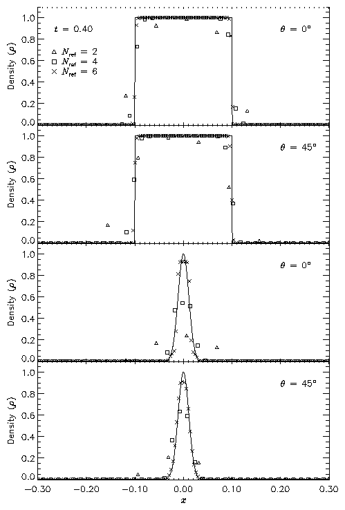
The advection results show the expected improvement with increasing AMR refinement level N_ref. Inaccuracies appear as diffusive spreading, rounding of sharp corners, and clipping. In both the square pulse and Gaussian pulse tests, diffusive spreading is limited to about one zone on either side of the pulse. For N_ref=2 the rounding of the square pulse and the clipping of the Gaussian pulse are quite severe; in the latter case the pulse itself spans about two zones, which is the approximate smoothing length in PPM for a single discontinuity. For N_ref=4 the treatment of the square pulse is significantly better, but the amplitude of the Gaussian is still reduced by about 50%. In this case the square pulse discontinuities are still being resolved with 2-3 zones, but the zones are now a factor of 25 smaller than the pulse width. With six levels of refinement the same behavior is observed for the square pulse, while the amplitude of the Gaussian pulse is now 93% of its initial value. The absence of dispersive effects (ie. oscillation) despite the high order of the PPM interpolants is due to the enforcement of monotonicity in the PPM algorithm.

The diagonal runs are consistent with the runs which were parallel to the x-axis, with the possibility of a slight amount of extra spreading behind the pulse. However, note that we have determined density values for the diagonal runs by interpolation along the grid diagonal. The interpolation points are not centered on the pulses, so the density does not always take on its maximum value (particularly in the lowest-resolution case).

These results are consistent with earlier studies of linear advection with PPM (e.g., Zalesak 1987). They suggest that, in order to preserve narrow flow features in FLASH, the maximum AMR refinement level should be chosen so that zones in refined regions are at least a factor 5-10 smaller than the narrowest features of interest. In cases in which the features are generated by shocks (rather than moving with the fluid), the resolution requirement is not as severe, as errors generated in the preshock region are driven into the shock rather than accumulating as it propagates.

5.6  The problem of a wind tunnel with a step

The problem of a wind tunnel containing a step was first described by Emery (1968), who used it to compare several hydrodynamical methods which are only of historical interest now. Woodward and Colella (1984) later used it to compare several more advanced methods, including PPM. Although it has no analytical solution, this problem is useful because it exercises a code's ability to handle unsteady shock interactions in multiple dimensions. It also provides an example of the use of FLASH to solve problems with irregular boundaries.

The problem uses a two-dimensional rectangular domain three units wide and one unit high. Between x=0.6 and x=3 along the x-axis is a step 0.2 units high. The step is treated as a reflecting boundary, as are the lower and upper boundaries in the y direction. For the right-hand x boundary we use an outflow (zero gradient) boundary condition, while on the left-hand side we use an inflow boundary. In the inflow boundary zones we set the density to r₀, the pressure to p₀, and the velocity to u₀, with the latter directed parallel to the x-axis. The domain itself is also initialized with these values. For the Emery problem we use

r0 = 1.4        p0 = 1        g = 1.4        u0 = 3 ,

(47)

which corresponds to a Mach 3 flow. Because the outflow is supersonic throughout the calculation, we do not expect reflections from the right-hand boundary.

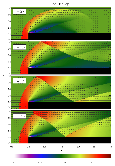
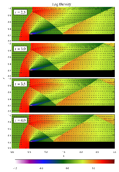
The additional runtime parameters supplied with the windtunnel problem are listed in Table 9. This problem is configured to use the perfect-gas equation of state (gamma) with gamma set to 1.4. We also set xmax=3, ymax=1, Nblockx=15, and Nblocky=4 in order to create a grid with the correct dimensions. The version of divide_domain supplied with this problem adds three top-level blocks along the lower left-hand corner of the grid to cover the region in front of the step. Finally, we use xlboundary=-23 (user boundary condition) and xrboundary=-21 (outflow boundary) to instruct FLASH to use the correct boundary conditions in the x direction. Boundaries in the y direction are reflecting (-20).

Until t=12 the flow is unsteady, exhibiting multiple shock reflections and interactions between different types of discontinuity. Figure 20 shows the evolution of density and velocity between t=0 and t=4 (the period considered by Woodward and Colella). Immediately a shock forms directly in front of the step and begins to move slowly away from it. Simultaneously the shock curves around the corner of the step, extending farther downstream and growing in size until it strikes the upper boundary just after t=0.5. The corner of the step becomes a singular point, with a rarefaction fan connecting the still gas just above the step to the shocked gas in front of it. Entropy errors generated in the vicinity of this singular point produce a numerical boundary layer about one zone thick along the surface of the step. Woodward and Colella reduce this effect by resetting the zones immediately behind the corner to conserve entropy and the sum of enthalpy and specific kinetic energy through the rarefaction. However, we are less interested here in reproducing the exact solution than in verifying the code and examining the behavior of such numerical effects as resolution is increased, so we do not apply this additional boundary condition. The errors near the corner result in a slight overexpansion of the gas there and a weak oblique shock where this gas flows back toward the step. At all resolutions we also see interactions between the numerical boundary layer and the reflected shocks which appear later in the calculation.

By t=1 the shock reflected from the upper wall has moved downward and has almost struck the top of the step. The intersection between the primary and reflected shocks begins at x » 1.45 when the reflection first forms at t » 0.65, then moves to the left, reaching x » 0.95 at t=1. As it moves, the angle between the incident shock and the wall increases until t=1.5, at which point it exceeds the maximum angle for regular reflection (40^° for g = 1.4) and begins to form a Mach stem. Meanwhile the reflected shock has itself reflected from the top of the step, and here too the point of intersection moves leftward, reaching x » 1.65 by t=2. The second reflection propagates back toward the top of the grid, reaching it at t=2.5 and forming a third reflection. By this time in low-resolution runs we see a second Mach stem forming at the shock reflection from the top of the step; this results from the interaction of the shock with the numerical boundary layer, which causes the angle of incidence to increase faster than in the converged solution. Figure 21 compares the density field at t=4 as computed by FLASH using several different maximum levels of refinement. Note that the size of the artificial Mach reflection diminishes as resolution improves.

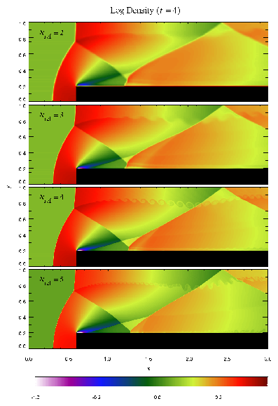
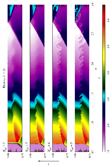
The shear zone behind the first (``real'') Mach stem produces another interesting numerical effect, visible at t=3 and t=4: Kelvin-Helmholtz amplification of numerical errors generated at the shock intersection. The wave thus generated propagates downstream and is refracted by the second and third reflected shocks. This effect is also seen in the calculations of Woodward and Colella, although their resolution was too low to capture the detailed eddy structure we see. Figure 22 shows the detail of this structure at t=3 on grids with several different levels of refinement. The effect does not disappear with increasing resolution, for two reasons. First, the instability amplifies numerical errors generated at the shock intersection, no matter how small. Second, PPM captures the slowly moving, nearly vertical Mach stem with only 1-2 zones on any grid, so as it moves from one column of zones to the next, artificial kinks form near the intersection, providing the seed perturbation for the instability. This effect can be reduced by using a small amount of extra dissipation to smear out the shock, as discussed by Colella and Woodward (1984). This tendency of physical instabilities to amplify numerical noise vividly demonstrates the need to exercise caution when interpreting features in supposedly converged calculations.

Finally, we note that in high-resolution runs with FLASH we also see some Kelvin-Helmholtz rollup at the numerical boundary layer along the top of the step. This is not present in Woodward and Colella's calculation, presumably because their grid resolution is lower (corresponding to two levels of refinement for us) and because of their special treatment of the singular point.

6  Going further with FLASH

FLASH is designed to be easy to configure, use, and extend. Configuration and use involve selecting particular sets of initial and boundary conditions, physics modules, and solution algorithms, as well as setting the values of parameters which control the simulation. Extension involves the addition of new problems, physics, and algorithms to suit the user's requirements. In this section we describe in some detail the structure of the FLASH source code, the format of the configuration files, and the runtime parameters and output formats available. We also discuss the steps a user needs to take in order to customize the code.

6.1  The FLASH code architecture

An abstract representation of the first-generation FLASH code architecture appears in Figure 23. In this figure, solid lines with triangles denote inheritance relationships, while dashed lines indicate instantiation relationships. Each box represents a class, which supplies data structures to its subclasses and methods to its calling classes. Italicized method names represent virtual functions, which are satisfied by subclasses. As this figure shows, the driver module controls the principal data structures used by the code, making them available to solver objects that it instantiates from the various classes of physics solvers. For time-dependent problems, the driver uses time-splitting techniques to compose the different solvers. The solvers are divided into different classes on the basis of their ability to be composed in this fashion and upon natural differences in solution method (e.g., hyperbolic solvers for hydrodynamics, elliptic solvers for radiation and gravity, ODE solvers for source terms, etc.). The adaptive mesh refinement library is treated in the same way as the solvers. The means by which the driver shares data with the solver objects is the primary way in which the architecture affects the overall performance of the code. Choices here, in order of decreasing performance and increasing flexibility, include global memory, argument-passing, and messaging. For historical reasons, and for the sake of performance, FLASH 1.x uses global memory to manage many of these interfaces.

The codes we have brought together in FLASH - including the PROMETHEUS hydrodynamical solver, specialized equation-of-state and nuclear burning codes, and the PARAMESH adaptive mesh refinement library - were written primarily in FORTRAN 77. This language, while efficient, does not by itself support objects or many of the other features needed to construct a modular architecture. However, Fortran 90 does offer some object capability, and it provides a straightforward migration path from FORTRAN 77, since the latter is a subset of the former. Thus we chose Fortran 90 as the integration language for FLASH 1.x. Using the module capability of Fortran 90, we have replaced many of the formerly global data structures in FLASH (e.g., runtime parameters) with container classes that provide externally visible accessor methods. This allows solvers to access global information on their own terms without having to declare common variables. The global memory associated with the mesh data structure has been retained in FLASH 1.x, but FLASH 2.0, currently being tested, replaces this too with an appropriate container class.

While Fortran 90 provides some object-oriented features (Decyk, Norton, & Szymanski 1997), it does not support true inheritance or polymorphism. This limits its runtime flexibility and requires us to set class relationships at compilation instead - a procedure that is feasible only if compilation is relatively fast, as it is for FLASH. In any case, configuring FLASH at compilation time makes it much easier for the compiler to produce aggressively optimized code, since it does not have to anticipate all possible class interactions.

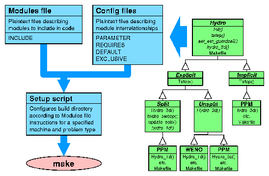
To provide inheritance and polymorphism at compilation we have created a configuration system consisting of a configuration script and several plaintext configuration files (one for each class) that describe the relationships between classes and subclasses - for example, which of the other classes a given class requires in order to function. The source code and configuration files for the classes are stored in a directory structure that corresponds directly to the class structure. The user specifies the classes to include in the code via a plaintext file that is taken as input by the configuration script. The script then parses the appropriate configuration files, constructing a build directory containing the requested source code, checking along the way for illegal combinations or missing requirements. The setup script also constructs makefiles for the different classes by concatenating makefile fragments supplied by each subclass. It then generates a master makefile that calls the various class makefiles. After running the setup script, the user builds the code by invoking gmake. A schematic representation of this procedure appears in Figure 24.

6.1.1  Code infrastructure

The structure of the FLASH source tree reflects the class structure of the code, as shown in Figure 25. The general plan is that source code is organized into one set of directories, while the code is built in a separate directory using links to the appropriate source files. The links are created by a source configuration script called setup, which makes the links using options selected by the user and then creates an appropriate makefile in the build directory. The user then builds the executable with a single invocation of gmake.

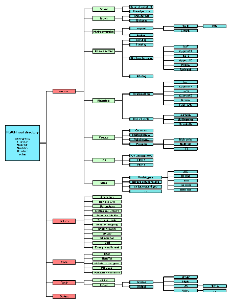
Source code for each of the different code modules is stored in subdirectories under source/. The code modules implement different physics, such as hydrodynamics, nuclear burning, and gravity, or different major program components, such as the main driver code and the input/output code. Each module directory contains source code files, makefile fragments indicating how to build the module, and a configuration file (see Section 6.1.2).

Each module subdirectory may also have additional sub-module directories underneath it. These contain code, makefiles, and configuration files specific to different variants of the module. For example, the hydro/ module directory can contain files which are generic to hydrodynamical solvers, while its explicit/ subdirectory contains files specific to explicit hydro schemes and its implicit/ subdirectory contains files specific to implicit solvers. Configuration files for other modules which need hydrodynamics can specify hydro as a requirement without mentioning a specific solver; the user can then choose one solver or the other when building the code (via the Modules file; Section 6.1.3). When setup configures the source tree it treats each sub-module as inheriting all of the source code, configuration files, and makefiles in its parent module's directory, so generic code does not have to be duplicated. Sub-modules can themselves have sub-modules, so for example one might have hydro/explicit/split/ppm and hydro/implicit/ppm. Source files at a given level of the directory hierarchy override files with the same name at higher levels, whereas makefiles and configuration files are cumulative. This permits modules to supply stub routines that are treated as `virtual functions' to be overridden by specific sub-modules, and it permits sub-module directories to be self-contained.

When a module is not explicitly included by Modules, only one thing is done differently by setup: sub-modules are not included, except for a null sub-module, if it is present. Most top-level modules should contain only stub files to be overridden by sub-modules, so this behavior allows the module to be `not included' without extra machinery (such as the special stub files and makefiles required by earlier versions of FLASH). In those cases in which the module's files are not appropriate for the `not included' case, the null sub-module allows one to override them with appropriate versions.

New solvers and new physics can be added. At the current stage of development of FLASH it is probably best to consult the authors of FLASH (see Section 7) for assistance in this. Some general guidelines for adding solvers to FLASH 1.6 may be found in Section 6.1.5 and Section 6.4.

An additional subdirectory of source/ called sites/ contains code specific to different installations (eg., sphere.uchicago.edu), each of which has its own directory. Each of these directories contains a makefile fragment called Makefile.h that is used to set machine-dependent compilation flags and so forth. In addition, special versions of any routines which are needed for each architecture are included in these directories. In future versions of FLASH we expect to generate site-dependent directories using the GNU configure command.

The setups/ directory has a structure similar to that of source/. In this case, however, each of the ``modules'' represents a different initial model or problem, and the problems are mutually exclusive; only one is included in the code at a time. Also, the problem directories have no equivalent of sub-modules. A makefile fragment specific to a problem need not be present, but if it is, it is called Makefile. Section 6.3 describes how to add new problem directories.

The setup script creates a directory called object/ in which the executable is built. In this directory setup creates links to all of the source code files found in the specified module and sub-module directories as well as the specified problem directory. (A source code file has the extension .c, .C, .f90, .F90, .f, .F, .fh, or .h.) Because the problem setup directory and the machine-dependent directory are scanned last, links to files in these directories override the ``defaults'' taken from the source/ tree. Hence special variants of routines needed for a particular problem can be used in place of the standard versions by simply giving the files containing them the same names.

Using information from the configuration files in the specified module and problem directories, setup creates a file named init_global_parms.f90 to parse the runtime parameter file and initialize the runtime parameter database. It also creates a file named rt_parms.txt, which concatenates all of the PARAMETER statements found in the appropriate configuration files and so can be used as a ``master list'' of all of the runtime parameters available to the executable.

setup also creates makefiles in object/ for each of the included modules. Each copy is named Makefile.module, where module is driver, hydro, gravity, and so forth. Each of these files is constructed by concatenating the makefiles found in each included module path. So, for example, including hydro/explicit/split/ppm causes Makefile.hydro to be generated from files named Makefile in hydro/, hydro/explicit/, hydro/explicit/split/, and hydro/explicit/split/ppm/. If the module is not explicitly included, then only hydro/Makefile is used, under the assumption that the subroutines at this level are to be used when the module is not included. The setup script creates a master makefile (Makefile) in object/ which includes all of the different modules' makefile fragments together with the site- or operating system-dependent Makefile.h.

The master makefile created by setup creates a temporary subroutine, buildstamp.f, which echoes the date, time, and location of the build to the FLASH log file when FLASH is run. To ensure that this subroutine is regenerated each time the executable is linked, the makefile deletes buildstamp.f immediately after compiling it.

The setup script can be run with the -portable option to create a directory with real files which can be collected together with tar and moved elsewhere for building. In this case the build directory is assigned the name object_problem/. Further information on the options available with setup may be found in Section 4.1.

Additional directories included with FLASH are tools/, which contains tools for working with FLASH and its output (Section 4), and docs/, which contains documentation for FLASH (including this user's guide) and the PARAMESH library.

6.1.2  Configuration files

Information about module dependencies, default sub-modules, runtime parameter definitions, and so on is stored in plain text files named Config in the different module directories. These are parsed by setup when configuring the source tree and are used to create the Fortran code needed to implement the runtime parameters, choose sub-modules when only a generic module has been specified, prevent mutually exclusive modules from being included together, and to flag problems when dependencies are not resolved by some included module. In the future they may contain additional information about module interrelationships. An example Config file appears in Figure 26.

# Configuration file for hydro module DEFAULT explicit EXCLUSIVE explicit implicit REQUIRES driver/time_dep REQUIRES materials/eos REQUIRES mesh PARAMETER eint_switch REAL 1.e-4      # below this cutoff, use internal energy from evolution equation

The syntax of the configuration files is as follows. Arbitrarily many spaces and/or tabs may be used, but all keywords must be in uppercase. Lines not matching an admissible pattern are ignored. (Someday soon they will generate a syntax error.)

6.1.3  Module files

The Modules file, which is created in the FLASH root directory either by the user or by setup -defaults, is used by setup to specify the particular code modules (and sub-modules) to include. It allows the user to combine desired variants of the different code modules or to use different solution algorithms while still satisfying the dependencies of the different modules. The setup script terminates with an error if all of the dependencies of the different included modules are not satisfied by some other included module. The format of this file is similar to that of the configuration files (Section 6.1.2), but only two types of instruction are recognized:

6.1.4  Runtime parameters

Runtime parameters are used to control the initial model, the various physics modules, and the behavior of the simulation. They are made available to FLASH via the setup configuration files described in Section 6.1.2. Their values can be set at runtime through the runtime parameter file and can be changed without requiring the user to rebuild the executable.

The runtime parameter file is a plain text file with the following format. Each line is either a comment (denoted by a hash mark, #), blank, or of the form variable = value. String values are enclosed in double quotes ("). Boolean values are indicated in the Fortran style, .true. or .false. Comments may appear at the end of a variable assignment line. An example parameter file may be found in Figure 1.

By default FLASH looks for a parameter file named flash.par in the directory from which it is run. An alternative file name can be specified as a command-line argument when FLASH is run.

In Section 6.1.5, Tables 11-16 list the runtime parameters made available by the different code modules included with FLASH. Please see Section 5 for more information on runtime parameters specific to each of the test problems supplied with FLASH.

6.1.5  Code modules

Currently this section is out-of-date. It refers to FLASH 1.0. However, it should still be helpful in understanding FLASH 1.6.

In this section we describe in turn each of the code modules included with FLASH, together with its available sub-modules and runtime parameters. We also discuss the ways in which new solvers or new physics modules must interact with each module in order to work with FLASH 1.0. Tables 11-16 list the runtime parameters for each module. More detailed descriptions of the algorithms included with FLASH may be found in Section 3.

Driver module (driver)

This module contains the main program and administrative subroutines which are not tied to any specific physics module. The driver module in FLASH 1.0 is oriented toward hyperbolic problems. Hence its major functions include setting initial conditions, calling output routines (which are handled by the io module) periodically, and managing the forward time advance of the simulation (including the calculation of the timestep).

The driver module also provides the global data context for FLASH. Most physics modules access this context by including the file common.fh, which itself includes the other include files needed by the driver (hence these other files need not be explicitly included). Since common.fh and its brethren use preprocessor statements, subroutines which include it have

#include "common.fh"

readparm.fh, which contains declarations needed by the runtime parameter parser, including the runtime parameter buffers;

rt_vars.fh, which is generated by setup and includes all runtime parameter declarations, their default settings, and their equivalences to the runtime parameter buffers;

constants.fh, which contains declarations and settings for physical constants;

definitions.fh, which contains code constant declarations;

physicaldata.fh, tree.fh, workspace.fh, and block_boundary_data.fh, which contain constant and array declarations for the block-structured mesh data structure used by the code; and

mpif.h, which contains Fortran constant declarations for use with the Message-Passing Interface library. This file is provided as part of the MPI distribution, not with FLASH.

The main program is contained in the file flash.F. It first reads the runtime parameter file and initializes the AMR library and physics modules. Then, depending upon the setting of the restart parameter, it calls init_from_scratch() to initialize the grid using the specified initial conditions or init_from_checkpoint() to read the initial conditions from a checkpoint file. The most important functions carried out by init_from_scratch() are the call to divide_domain(), which allocates top-level AMR blocks, and the call to init_block(), which initializes a single block (and is part of the hydro module). All problem setups must provide a version of init_block(). On the other hand, the divide_domain() subroutine provided with FLASH is fairly general and can set up a top-level mesh with Nblockx×Nblocky× Nblockz blocks. For irregular domains (such as in the windtunnel test problem), a special version of divide_domain() should be provided as part of the problem setup. (See Section 6.3 for a discussion of creating new problem setups. The files containing the replacement routines should be given the same names as the originals.)

After initialization the main program calls output_initial() (part of the io module) to write a checkpoint file containing the initial conditions and to create the scalar/global file, to which FLASH writes the total energy and other quantities at the end of each timestep.

Following the initial output in flash.F is the main evolution loop, consisting of a call to hydro_3d() (which advances the system one timestep), a call to timestep() (which determines the size of the next timestep according to constraints provided by each of the solver modules), and a call to output() (which writes to the scalar/global file and produces checkpoint files at specified intervals). In FLASH 1.0 the evolution routine hydro_3d() is part of the hydro module, which is essentially the evolution part of the PROMETHEUS code (Section 3.1). The loop terminates either when nend timesteps have been taken or when the simulation time exceeds tmax. The last things the main program does are to checkpoint the final timestep and print CPU timing information.

Currently the hydrodynamics, equation of state, gravity, and nuclear burning routines are all called from within hydro_3d(). In FLASH 1.5 the evolution function is taken over from hydro_3d() by a routine called evolve() which is part of the driver module. However, since evolution in FLASH 1.0 is handled by a routine which is properly part of the hydro module, FLASH 1.0 should always be built with hydrodynamics included. (Alternatively, a new non-hydro physics module might supply a replacement for hydro_3d().) Users wishing to implement new physics modules within FLASH 1.0 should insert calls to their solver routines in hydro_3d(). In order to access the block-structured mesh data, global variables (such as the simulation time and the number of processors), and runtime parameters, new module routines should include common.fh as discussed above. With the data structure and modularity enhancements coming in FLASH 1.5 we expect the process of adding a new solver to become much simpler. See Section 6.4 for further general guidelines on adding solvers to FLASH.

Hydrodynamics module (hydro)

The hydro module solves the Euler equations of hydrodynamics (see Section 3.1). The solver included with FLASH 1.0 is directionally split and is based on the piecewise-parabolic method (PPM; Colella & Woodward 1984). Future versions will include sub-modules to handle unsplit PPM and perhaps other hydro algorithms.

As discussed in the previous section, in its current form the hydro module handles the evolution function of the driver module through the routine hydro_3d(). This routine performs one-dimensional sweeps in the x, y, and z directions, calls the nuclear burning routine (burn()), and then applies these operators in reverse order. Hydrodynamical boundary conditions are set before each 1D sweep by a call to the PARAMESH routine amr_guardcell(). For each sweep, the code cycles through the leaf-node blocks, applying the 1D hydro operator to each in turn. For a single block, hydro_3d() loops over the coordinates transverse to the sweep direction, copying rows of data from the block array to a 1D sweep array (via getrwx(), getrwy(), and getrwz()). For each row, hydrodynamical fluxes are computed with a call to hydrow(); these fluxes are then used to update zones in the interior of the block with update_soln() and in the guard cells with update_soln_boun(). Following the application of each 1D hydrodynamical operator, the hydrodynamical fluxes are corrected to ensure conservation at jumps in refinement with a call to the PARAMESH routine amr_flux_conserve(). At the end hydro_3d() tests the grid refinement with several calls to the PARAMESH amr_test_refinement() routine, then initiates changes in refinement with a call to the PARAMESH amr_refine_derefine() routine.

Three other externally visible routines in the hydro module are init_hydro(), which initializes the module by setting the hydrodynamical variables to zero; init_block(), which sets the initial conditions in a single block; and tot_bnd(), which is called by the PARAMESH guard cell filling routines when an external boundary is encountered. The latter two routines are the most important from the standpoint of users wishing to construct a new problem setup (Section 6.3).

In addition to the global common file common.fh, the hydrodynamical routines include three other common files: common_hydro.fh, which contains declarations for variables specific to 1D hydrodynamical schemes (appropriate to the operator-split implementation in FLASH 1.0); common_ppm.fh, which contains declarations specific to the piecewise-parabolic method; and iso13.fh, the common file exported by the nuclear burning module and containing information on the nuclear isotopes to track (only used by hydro_3d()).

Equation of state module (eos)

The eos module implements the equation of state needed by the hydrodynamical and nuclear burning solvers. Three sub-modules are available in FLASH 1.0: gamma, which implements a perfect-gas equation of state; nadozhin, which implements an equation of state appropriate to partially degenerate material at nuclear densities in thermal equilibrium with radiation (Nadyozhin 1974); and helmholtz, which uses a fast Helmholtz free-energy table interpolation to handle the same physics as nadozhin (Timmes & Swesty 1999).

The primary interface routine for the eos module in FLASH 1.0 is eos3d(), which sets the pressure in an entire block of zones by calling the eos() routine supplied by each equation of state sub-module. The input data for this routine are the density, temperature, and thermal energy for the block (the block's local identification number is passed as an argument, and the block data are referenced through the global common blocks). Usually eos3d() is called when these values have been changed (e.g., by the hydro routines) and the pressure must be made consistent with them again. The eos() routine performs this computation for a row of zones. (Routines in the eos module include common files exported by the hydro and burn modules. For this [and physics] reasons, sensible use of eos requires the hydro module [and, for nadozhin and helmholtz, the burn module] to be included.) Each sub-module also supplies a routine called eos_fcn() which enables the pressure to be returned for specified values of the density, temperature, energy, and composition, without reference to the grid.

Nuclear burning module (burn)

The nuclear burning module uses a sparse-matrix semi-implicit ordinary differential equation (ODE) solver to calculate the nuclear burning rate and update the fluid variables accordingly (Timmes 1999). The primary interface routines for this module are init_burn(), which calls routines to set up the nuclear isotope tables needed by the module; and burn(), which calls the ODE solver and updates the hydrodynamical variables in a single row of a single AMR block. In addition to the global common file common.fh and the 1D hydrodynamical common file common_hydro.fh, the burning routines include a common file named iso13.fh which declares variables shared within the burning module.

Gravity module (grav)

The grav module sets up the gravitational field; the effects of gravity are handled by the hydro module. In FLASH 1.0 the only gravitational field sub-module is constant, which creates a uniform acceleration in the x-direction. The next version of FLASH will include a Poisson solver to compute the gravitational field due to the matter on the computational grid. This module supplies two routines: gravty(), which sets the gravitational acceleration in a row of zones, and tstep_grav(), which sets the timestep constraint due to gravitation (currently a no-op).

Input/output module (io)

The io module handles the output produced by FLASH, in particular the periodic checkpoints and the regular output of total energy, mass, and momentum information. It has two sub-modules, hdf, which selects the Hierarchical Data Format (HDF) for checkpoint files, and f77_unf, which selects Fortran 77 unformatted output. The HDF output produced by io/hdf is described in Section 6.2.

The primary interface routines for the io module are output_initial(), which handles output just after initialization and before the main FLASH timestep loop is entered; output(), which handles periodic output inside the timestep loop; output_final(), which handles output following the completion of the timestep loop; and wr_integrals(), which computes the totals of several quantities, including energy, mass, momentum, and so on, then writes them to an (ASC)I file named flash.dat at the end of each timestep. The checkpoint routines provided by the two sub-modules of io are checkpoint_wr(), which writes checkpoint files, and checkpoint_re(), which reads them in.

PARAMESH and related modules (paramesh, mmpi, mpi_amr)

The paramesh module supplies the adaptive mesh-refinement (AMR) library used by the rest of FLASH (MacNeice et al. 1999). It supplies a block-structured grid with factor-of-two refinement between levels, as described in Section 3.2. The mmpi and mpi_amr modules supply routines for translating the shared-memory subroutine calls used by PARAMESH into Message-Passing Interface (MPI) calls. The next version of PARAMESH, which will be included with a future version of FLASH, relies only upon MPI calls, and these modules will cease to be included. See the PARAMESH home page at

http://esdcd.gsfc.nasa.gov/ESS/macneice/paramesh/paramesh.html

6.2  Formats of output files produced by FLASH

Currently FLASH can store simulation data in three basic formats: F77, HDF 4, and HDF 5. Different techniques can be used to write the data: moving all the data to a single processor for output; each processor writing to a separate file; and parallel access to a single file. The output format varies from module to module, and is described here in detail.

The default I/O module is Hierarchical Data Format version 4 (HDF 4). This HDF format provides an API for organizing data in a database fashion. In addition to the raw data, information about the data type and byte ordering (little or big endian), rank, and dimensions of the dataset is stored. This makes the HDF format extremely portable. Different packages can query the file for its contents, without knowing the details of the routine that generated the data.

HDF 4 is limited to files < 2 GB is size. Furthermore, the official release of HDF 4 does not support parallel I/O. To address these limitations, HDF 5 was released. HDF 5 is supported on a large variety of platforms, and offers the same functionality as HDF 4, with the addition of large file support and parallel I/O via MPI-I/O. Information of the different versions of HDF can be found at http://hdf.nsca.uiuc.edu. This section assumes that you already have the necessary HDF libraries installed on your machine.

The I/O modules in FLASH have two responsibilities-generating and restarting from checkpoint files, and generating plot files. A checkpoint file contains all the information needed to restart the simulation. The data is stored at the same precision (8-byte reals) as it is carried in the code. A plotfile contains all the information needed to interpret the tree structure maintained by FLASH and it contains a user-defined subset of the variables. Furthermore, the data may be stored at reduced precision to conserve space.

The type of output you create will depend on what type of machine you are running on, the size of the resulting dataset, and what you plan on doing with the datafiles once created. Table 17 summarizes the different modules which come with FLASH.

6.2.1  General parameters

There are several parameters that control the frequency of output, type of output, and name of the output files. These parameters are the same for all the different modules, although not every module is required to implement all parameters. These parameters are used in the top level I/O routines (initout.F, output.F, and finalout.F) to determine when to output. Some parameters are used to determine the resulting filename. Table 18 gives a description of the I/O parameters.

6.2.2  Output file names

FLASH constructs the output filenames based on the user-supplied basename and the file counter that is incremented after each output. Additionally, information about the file type and data storage is included in the filename.
 
The general checkpoint filename is:
basename_{

hdf

hdf5

f77

}_chk_0000,
where hdf, hdf5, or f77 is picked depending on the I/O module used and the number at the end of the filename is the current cpnumber.
 
The general plotfile filename is:
basename_{

hdf

hdf5

f77

}_plt_{

crn

cnt

}_0000,
where hdf, hdf5, or f77 is picked depending on the I/O module used, crn and cnt indicate data stored at the cell corners or centers respectively, and the number at the end of the filename is the current ptnumber.

6.2.3  HDF 4

The HDF 4 output module creates a single file containing the data on all processors, if the total size of the dataset is < 2 GB. If there is more than 2 GB of data to be written, multiple files are created to store the data. The number of files used to store the dataset is contained in the number of files record. Each file contains a subset of the blocks (stored in the local blocks record) out of the total number of blocks in the simulation. The blocks are divided along processor boundaries.

The HDF 4 module performs serial I/O-each processors data is moved to the master processor to be written to disk. This has the advantage of producing a single file for the entire simulation, but is less efficient than if each processor wrote to disk.

HDF 4 has been tested successfully on most machines, with the exception of (ASC) Red.

Table 19 summarizes the records stored in a HDF 4 file. The format of the plotfiles and checkpoint files are the same, with the only difference being the number of unknowns stored. The records contained in a HDF 4 file can be found via the hdp command that is part of the HDF 4 distribution. The syntax is hdp dumpsds -h filename. The contents of a record can be output by hdp dumpsds -i N filename, where N is the index of the record.

As described above, HDF 4 cannot produce files > 2 GB in size. This is overcome in the FLASH HDF 4 module by splitting the dataset into multiple files when it would otherwise produce a file larger than 2 GB in size.

When reading a single unknown from a FLASH HDF 4 file, you will suffer performance penalties, as there will be many non-unit-stride accesses on the first dimension, since all the variables are stored together in the file.

Table 20: FLASH HDF 4 file format.
Record label	Description of the record
Table 21: HDF 4 format (continued).
Record label	Description of the record
file creation time	character*40 file_creation_time
	The time and date that the file was created.
total blocks	integer tot_blocks
	The total number of blocks in the simulation.
	Note: the number of blocks contained in this file may be less than the total number of blocks if the output is spread across multiple files (see `number of files' and `local blocks')
time	real time
	The simulation time at file output.
timestep	real dt
	The current timestep.
number of steps	integer nsteps
	The number of timesteps from the start of the calculation.
number of blocks per zone	real nblocks_per_zone(3)
	The number of zones in each direction:
	nblocks_per_zone(1) - x-direction
	nblocks_per_zone(2) - y-direction
	nblocks_per_zone(3) - z-direction
number of files	integer num_files
	The number of files that comprise the dataset. Because the filesize cannot be larger than 2 GB, the data is split into multiple files if necessary, with each containing roughly the same number of blocks.
local blocks	integer local_blocks
	The number of blocks in this file. If there are multiple files, this number will be less than `total blocks'.
unknown names	character*4 unk_names(nvar)
	This array contains 4 character names corresponding to the first index of the unk array. They serve to identify the variables stored in the `unknowns' record.
refine level	integer lrefine(local_blocks)
	This array stores the refinement level for each block.
node type	integer nodetype(local_blocks)
	This array stores the nodetype for a block. Blocks with nodetype = 1 are leaf nodes, and this data will always be valid. For plotting purposes, it is the leaf data that you want to plot.
gid	integer gid(nfaces+1+nchild,local_blocks)
	This is the global identification array. For a given block, this array gives the block number of the blocks that neighbor it, and the block number of its parent and children.
	The first nfaces elements point to the neighbors (at the same level of refinement). The faces are numbered from minimum to maximum coordinate with x first, followed by y, and z. A -1 indicates that there is no neighbor at the same level of refinement. A number < = -20 indicates that you are on the physical boundary of the domain. If the neighbor points to the current block, it means that there are periodic boundary conditions. The next element points to the parent of the current block, and the last nchild elements point to the children of the current block.
	Ex: below is a simple domain, assume that at the boundaries, everything is -20
	looking at block no 5 (2-d):
	gid(1,block_no) = 4
	gid(2,block_no) = -1
	gid(3,block_no) = 3
	gid(4,block_no) = -20
	gid(5,block_no) = 1   (the parent)
	gid(6,block_no) = -1  (the children)
	gid(7,block_no) = -1
	gid(8,block_no) = -1
	gid(9,block_no) = -1
	looking at block no 1:
	gid(1,block_no) = -20
	gid(2,block_no) = 6
	gid(3,block_no) = -20
	gid(4,block_no) = -20
	gid(5,block_no) = -1
	gid(6,block_no) = 2
	gid(7,block_no) = 3
	gid(8,block_no) = 4
	gid(9,block_no) = 5
coordinates	real coord(ndim,local_blocks)
	This array stores the coordinates of the center of the block.
	coord(1,block_no) = x-coordinate
	coord(2,block_no) = y-coordinate
	coord(3,block_no) = z-coordinate
block size	real size(ndim,local_blocks)
	This array stores the dimensions of the current block.
	size(1,block_no) = x size
	size(2,block_no) = y size
	size(3,block_no) = z size
bounding box minimum	real bnd_box_min(ndim,local_blocks)
	This array stores the coordinate of the minimum block edge in each direction.
	bnd_box_min(1,block_no) = minimum x edge
	bnd_box_min(2,block_no) = minimum y edge
	bnd_box_min(3,block_no) = minimum z edge
bounding box maximum	as above, but the maximum edge value in each direction.
unknowns	real unk(nvar,nx,ny,nz,local_blocks)
	nx = no. of zones/block in x
	ny = no. of zones/block in y
	nz = no. of zones/block in z
	This array holds the unknowns. The variables corresponding to the first argument are listed in the `unknown names' record. Note, for a plot file with CORNERS=.TRUE. in the parameter file, the information is interpolated to the zone corners before being stored. This is useful for certain plotting packages.

6.2.4  HDF 5

There are two major HDF 5 modules, the serial and parallel versions. The format of the output file produced by these modules is identical, only the method by which it is written differs. Additionally, there are single precision versions of some of the modules, which produce plotfiles with 4-byte instead of 8-byte reals. At the time of this writing, the current version of HDF 5 is 5.1.2.2.

The HDF 5 modules have been tested successfully on the three (ASC) platforms. Performance varies widely across the platforms, and currently, HDF 5 use is only recommended on SGIs and (ASC) Blue Pacific.

The data format FLASH uses for HDF 5 output files is similar to that of the HDF 4 files, with the major difference in how the unknowns are stored. Instead of putting all the unknowns in a single HDF record, unk(nvar,nx,ny,nz,tot_blocks) as in the HDF 4 file, each variable is stored in its own record, labeled by the 4-character variable name. This allows for easier access to a single variable when reading from the file. The HDF 5 format is summarized in table 20.

Table 22: FLASH HDF 5 file format.
Record label	Description of the record
Table 23: HDF 5 format (continued).
Record label	Description of the record
file creation time	character*40 file_creation_time
	The time and date that the file was created.
total blocks	integer tot_blocks
	The total number of blocks in the simulation.
time	real time
	The simulation time at file output.
timestep	real dt
	The current timestep.
number of steps	integer nsteps
	The number of timesteps from the start of the calculation.
number of zones per block	real nblocks_per_zone(3)
	The number of zones in each direction:
	nblocks_per_zone(1) - x-direction
	nblocks_per_zone(2) - y-direction
	nblocks_per_zone(3) - z-direction
unknown names	character*4 unk_names(nvar)
	This array contains 4 character names corresponding to the first index of the unk array. They serve to identify the variables stored in the `unknowns' record.
refine level	integer lrefine(tot_blocks)
	This array stores the refinement level for each block.
node type	integer nodetype(tot_blocks)
	This array stores the nodetype for a block. Blocks with nodetype = 1 are leaf nodes, and this data will always be valid. For plotting purposes, it is the leaf data that you want to plot.
gid	integer gid(nfaces+1+nchild,tot_blocks)
	This is the global identification array. For a given block, this array gives the block number of the blocks that neighbor it, and the block number of its parent and children.
	see the description in the HDF 4 table for full details.
coordinates	real coord(ndim,tot_blocks)
	This array stores the coordinates of the center of the block.
	coord(1,block_no) = x-coordinate
	coord(2,block_no) = y-coordinate
	coord(3,block_no) = z-coordinate
block size	real size(ndim,tot_blocks)
	This array stores the dimensions of the current block.
	size(1,block_no) = x size
	size(2,block_no) = y size
	size(3,block_no) = z size
bounding box minimum	real bnd_box_min(ndim,tot_blocks)
	This array stores the coordinate of the minimum block edge in each direction.
	bnd_box_min(1,block_no) = minimum x edge
	bnd_box_min(2,block_no) = minimum y edge
	bnd_box_min(3,block_no) = minimum z edge
bounding box maximum	as above, but the maximum edge value in each direction.
variable	real unk(nx,ny,nz,tot_blocks)
	nx = no. of zones/block in x
	ny = no. of zones/block in y
	nz = no. of zones/block in z
	This array holds the data for a single variable. The record label is identical to the 4-character variable name stored in the record unknown names. Note, for a plot file with CORNERS=.TRUE. in the parameter file, the information is interpolated to the zone corners and stored.

6.2.5  FORTRAN 77 (f77)

Unlike the HDF files, the f77 files do not have a record based format. This means it is necessary to know the precise way the data was written to disk, to construct the analogous read statement. In general, the data for a single block (tree, grid, and unknown information) is stored together in the file. The different f77 modules use different precision for the plotfiles, and this must be taken into account when reading the data.

The f77 modules with `_parallel' appended to the name create a single file from each processors, instead of first moving the data to processor 0 for writing. This is a lot faster on most platforms. It has the disadvantage of generating a lot of files, which must all be read in to recreate the dataset.

The f77_unf_parallel{_single} modules include a converter that will read in the header file for the plotfiles, and create a single HDF 5 plotfile containing all the data. This conversion routine is unsupported, but provided for completeness.

Working with output files

The HDF output formats offer the greatest flexibility when visualizing the data, as the visualization program does not have to know the details of how the file was written, rather it can query the file to find the datatype, rank, and dimensions. The HDF formats also avoid difficulties associated with different platforms storing numbers differently (big endian vs. little endian).

6.3  Creating new problems

In general, creating new sets of initial conditions is quite straightforward. Most users need only duplicate one of the existing setups and then edit it to suit their needs. Here we list the steps needed in order to create a new problem from scratch; at any step you may wish to copy a file from a similar existing setup and use it as a starting point. For example, to create a problem with plane-parallel symmetry, but in which the plane normal is adjustable, it may be helpful to start with files from the sod test problem. Similarly, for cylindrically or spherically symmetric initial conditions the sedov problem is a useful starting point.

1. Create a directory in setups/ with the name of the problem. Move to this directory.
2. Create a setup configuration file named Config. The format of this file is described in Section 6.1.2. This tells the setup script which optional code modules are required and which runtime parameters to create.
3. Create code files to set up the problem and do anything else needed. If hydrodynamics is included, at a minimum you must have a file named init_block.F, containing a subroutine named init_block() which sets up the density, pressure, velocity, etc. for the gas. If your problem requires special boundary conditions, you should also have a version of the file tot_bnd.F, which contains a routine to set the values of fluid variables in the guard cells. If your problem has an irregular boundary, you need a version of the file divide_domain.F, which creates the top-level AMR block structure. See one of the supplied problem setups for examples.

   For any files you create in the problem's setup directory with extensions .C, .c, .F, .f, .h, or .fh, the setup script will automatically create links in the object/ directory. However, they will only be compiled and linked into the executable if you create a makefile for the problem. Files such as init_block.F, which have the same name as a file in the included source directories, will simply replace the default files and do not require special treatment. For other files, create a short Makefile (call it that) in the problem setup directory with the contents

   #---special files for problem---
   problem = list of object files
   #---end special files-----

   where problem is the name of your problem.

6.4  Adding new solvers

Adding new solvers (either for new or existing physics) to FLASH is similar in some ways to adding a problem configuration. In general one creates a subdirectory for the solver, placing it under the source subdirectory for the parent module if the solver implements currently supported physics, or creating a new module subdirectory if it does not. Put the source files required by the solver into this directory, then create the following files:

Makefile: The make include file for the module should set a macro with the name of the module equal to a list of the object files in the module. Optionally (recommended), add a list of dependencies for each of the source files in the module. For example, the source_terms module's make include file is

# Makefile for source term solvers

source_terms = source_terms.o burn.o heat.o cool.o init_burn.o \
          init_heat.o init_cool.o tstep_burn.o tstep_heat.o \
          tstep_cool.o init_src.o

source_terms.o : source_terms.F common.fh
burn.o : burn.F
heat.o : heat.F
cool.o : cool.F
init_src.o : init_src.F common.fh
init_burn.o : init_burn.F
init_heat.o : init_heat.F
init_cool.o : init_cool.F
tstep_burn.o : tstep_burn.F
tstep_heat.o : tstep_heat.F
tstep_cool.o : tstep_cool.F

Sub-module make include files use macro concatenation to add to their parent modules' make include files. For example, the source_terms/burn sub-module has the following make include file:

# Makefile for the nuclear burning sub-module

source_terms += burn_block.o net_auxillary.o net_integrate.o \
           sparse_ma28.o gift.o net.o

burn_block.o : burn_block.F common.fh network_common.fh eos_common.fh
net_auxillary.o : net_auxillary.F network_common.fh eos_common.fh
net_integrate.o : net_integrate.F network_common.fh
sparse_ma28.o : sparse_ma28.F
net.o : net.F network_common.fh eos_common.fh
gift.o : gift.F

network_common.fh : network_size.fh
touch network_common.fh

# Additional dependencies

burn.o : common.fh network_common.fh
init_burn.o : common.fh network_common.fh

Note that the sub-module's make include file only makes reference to files provided at its own level of the directory hierarchy. If the sub-module provides special versions of routines to override those supplied by the parent module, they do not need to be mentioned again in the object list, because the sub-module's Makefile is contenated with its parent's. However, if these special versions have additional dependencies, they can be specified as shown. Of course, any files supplied by the sub-module that are not part of the parent module should be mentioned in the sub-module's object list, and their dependencies should be included.

If you are creating a new top-level module, your source files at this level will be included in the code even if you do not request the module in Modules. However, no sub-modules will be included. If you intend to have special versions of these files (stubs) that are used when the module is not included, create a sub-module named null and place them in it. null is automatically included if it is found and the module is not referenced in Modules.

If you create a top-level module with no Makefile, setup will automatically generate an empty one. For example, creating a directory named my_module/ in source/ causes setup to generate a Makefile.my_module in the build directory with contents

my_module =

If sub-modules of my_module exist and are requested, their Makefiles will be appended to this base.

In FLASH 1.6 it is no longer necessary to modify setup when adding a new top-level module. setup automatically scans the source/ directory for modules to use.

Config: Create a configuration file for the module or sub-module you are creating. All configuration files in a sub-module path are used by setup, so a sub-module inherits its parent module's configuration. Config should declare any runtime parameters you wish to make available to the code when this module is included. It should indicate which (if any) other modules your module requires in order to function, and it should indicate which (if any) of its sub-modules should be used as a default if none is specified when setup is run. The configuration file format is described in Section 6.1.2.

This is all that is necessary to add a module or sub-module to the code. However, it is not sufficient to have the module routines called by the code! If you are creating a new solver for an existing physics module, the module itself should provide the interface layer to the rest of the code. As long as your sub-module provides the routines expected by the interface layer, the sub-module should be ready to work. However, if you are adding a new module (or if your sub-module has externally visible routines - a no-no for the future), you will need to add calls to your externally visible routines. It is difficult to give completely general guidance; here we simply note a few things to keep in mind.

If you wish to be able to turn your module on or off without recompiling the code, create a new runtime parameter (e.g., use_module) in the driver module. You can then test the value of this parameter before calling your externally visible routines from the main code. For example, the burn module routines are only called if (iburn .eq. 1). (Of course, if the burn module is not included in the code, setting iburn to 1 will result in empty subroutine calls.)

You will need to add #include "common.fh" if you wish to have access to the global AMR data structure. Since this is the only mechanism for operating on the grid data (which is presumably what you want to do) in FLASH 1.x, you will probably want to do this. An alternative, if your module uses a pre-existing data structure, is to create an interface layer which converts the PARAMESH-inspired tree data structure used by FLASH into your data structure, then calls your routines. This will probably have some performance impact, but it will enable you to quickly get things working.

You may wish to create an initialization routine for your module which is called before anything (e.g., setting initial conditions) is done. In this case you should call the routine init_module() and place a call to it (without any arguments) in the main initialization routine, init_flash.F, which is part of the driver module. Be sure this routine has a stub available.

If your solver introduces a constraint on the timestep, you should create a routine named tstep_module() which computes this constraint. Add a call to this routine in timestep.F (part of the driver/time_dep module), using your global switch parameter if you have created one. See this file for examples. Your routine should operate on a single block and take three parameters: the timestep variable (a real variable which you should set to the smaller of itself and your constraint before returning), the minimum timestep location (an integer array with five elements), and the block identifier (an integer). Returning anything for the minimum location is optional, but the other timestep routines interpret it in the following way. The first three elements are set to the coordinates within the block of the zone contributing the minimum timestep. The fourth element is set to the block identifier, and the fifth is set to the current processor identifier (MyPE). This information tags along with the timestep constraint when blocks and solvers are compared across processors, and it is printed on stdout by the master processor along with the timestep information as FLASH advances.

If your solver is time-dependent, you will need to add a call to your solver in the evolve() routine (driver/time_dep/evolve.F). If it is time-independent, add the call to driver/steady/flash.F. evolve() implements second-order Strang time splitting within the time loop maintained by driver/time_dep/flash.F. The steady version of flash.F simply calls each operator once and then exits.

Try to limit the number of entry points to your module. This will make it easier to update it when the next version of FLASH is released. It will also help to keep you sane.

6.5  Porting FLASH to other machines

Porting FLASH to new architectures should be fairly straightforward for most Unix or Unix-like systems. For systems which look nothing like Unix, or which have no ability to interpret the setup script or makefiles, extensive reworking of the meta-code which configures and builds FLASH would be necessary. We do not treat such systems here; rather than do so, it would be simpler for us to do the port ourselves. The good news in such cases is that, assuming that you can get the source tree configured on your system and that you have a Fortran 90 compiler and the other requirements discussed in Section 2, you should be able to compile the code without making too many changes to the source. We have generally tried to stick to standard Fortran 90, avoiding machine-specific features.

For Unix-like systems, you should make sure that your system has csh, a gmake which permits included makefiles, awk, and sed. You will need to create a directory in source/sites/ with the name of your site (or a directory in source/sites/Prototypes/ with the name of your operating system). At a minimum this directory should contain a makefile fragment named Makefile.h. The best way to start is to copy one of the existing makefile fragments to your new directory and modify that. Makefile.h sets macros which define the names of your compilers, the compiler and linker flags, the names of additional object files needed for your machine but not included in the standard source distribution, and additional shell commands (such as file renaming and deletion commands) needed for processing the master makefile.

For most Unix systems this will be all you need to do. However, in addition to Makefile.h you may need to create machine-specific subroutines which override the defaults included with the main source code. As long as the files containing these routines duplicate the existing routines' filenames, they do not need to be added to the machine-dependent object list in Makefile.h; setup will automatically find the special routine in the system-specific directory and link to it rather than to the general routine in the main source directories.

An example of such a routine is getarg(), which returns command-line arguments and is used by FLASH to read the name of the runtime parameter file from the command line. This routine is not part of the Fortran 90 standard, but it is available on many Unix systems without the need to link to a special library. However, it is not available on the Cray T3E; instead, a routine named pxfgetarg() provides the same functionality. Therefore we have encapsulated the getarg() functionality in a routine named get_arguments(), which is part of the driver module in a file named getarg.f. The default version simply calls getarg(). For the T3E a replacement getarg.f calling pxfgetarg() is supplied. Since this file overrides a default file with the same name, getarg.o does not need to be added to the machine-dependent object list in source/sites/Prototypes/UNICOS/Makefile.h.

7  Contacting the authors of FLASH

FLASH is still under active development, so many desirable features have not yet been included (eg., self-gravity, thermal conduction, radiation transport, etc.). Also, you will most likely encounter bugs in the distributed code. A mailing list has been established for reporting problems with the distributed FLASH code. To report a bug, send email to

flash-bugs@mcs.anl.gov

giving your name and contact information and a description of the procedure you were following when you encountered the error. Information about the machine, operating system (uname -a), and compiler you are using is also extremely helpful. Please do not send checkpoint files, as these can be very large. If the problem can be reproduced with one of the standard test problems, send a copy of your runtime parameter file and your setup options. This situation is very desirable, as it limits the amount of back-and-forth communication needed for us to reproduce the problem. We cannot be responsible for problems which arise with a physics module or initial model you have developed yourself, but we will generally try to help with these if you can narrow down the problem to an easily reproducible effect which occurs in a short program run and if you are willing to supply your added source code.

At present no address has been set up for general development questions and comments, but we expect this to change in the near future. Documentation (including this user's guide) and support information for FLASH can be obtained on the World Wide Web at

http://flash.uchicago.edu/flashcode/

8  References

Aparicio, J. M. 1998, ApJS, 117, 627

Bader, G., Deuflhard, P. 1983, NuMat, 41, 373

Berger, M. J., Collela, P. 1989, JCP, 82, 64

Berger, M. J., Oliger, J. 1984, JCP, 53, 484

Blinnikov, S. I., Dunina-Barkovskaya, N. V.,, Nadyozhin, D. K. 1996, ApJS, 106, 171

Boris, J. P., Book, D. L. 1973, JCP, 11, 38

Burgers, J. M. 1969, Flow Equations for Composite Gases (New York: Academic)

Caughlan, G. R., Fowler, W. A. 1988, Atomic Data and Nuclear Data Tables, 40, 283

Chapman, S., Cowling, T. G. 1970, The Mathematical Theory of Non-uniform Gases (Cambridge: CUP)

Colella, P., Glaz, H. M. 1985, JCP, 59, 264

Colella, P., Woodward, P. 1984, JCP, 54, 174

Decyk, V. K., Norton, C. D.,, Szymanski, B. K. 1997, ACM Fortran Forum, 16 (also http://www.cs.rpi.edu/~szymansk/oof90.html)

DeZeeuw, D., Powell, K. G. 1993, JCP, 104, 56

Duff, I. S., Erisman, A. M.,, Reid, J. K. 1986, Direct Methods for Sparse Matrices (Oxford: Clarendon Press)

Emery, A. F. 1968, JCP, 2, 306

Fletcher, C. A. J. 1991, Computational Techniques for Fluid Dynamics, 2d ed. (Berlin: Springer-Verlag)

Forester, C. K. 1977, JCP, 23, 1

Fryxell, B. A., Müller, E.,, Arnett, D. 1989, in Numerical Methods in Astrophysics, ed. P. R. Woodward (New York: Academic)

Fryxell, B., Olson, K., Ricker, P., Timmes, F. X., Zingale, M., Lamb, D. Q., MacNeice, P., Rosner, R., Truran, J. W.,, Tufo, H. 2000, ApJS, 131, 273

Godunov, S. K. 1959, Mat. Sbornik, 47, 271

Itoh, N., Hayashi, H., Nishikawa, A.,, Kohyama, Y. 1996, ApJS, 102, 411

Khokhlov, A. M. 1997, Naval Research Lab memo 6406-97-7950

Löhner, R. 1987, Comp. Meth. App. Mech. Eng., 61, 323

MacNeice, P., Olson, K. M., Mobarry, C., de Fainchtein, R.,, Packer, C. 1999, CPC, accepted

Nadyozhin, D. K. 1974, Nauchnye informatsii Astron, Sov. USSR, 32, 33

Parashar M., 1999, private communication (http://www/caip.rutgers.edu/~parashar/DAGH)

Press, W. H., Teukolsky, S. A., Vetterling, W. T.,, Flannery, B. P. 1992, Numerical Recipes in Fortran, 2d ed. (Cambridge: CUP)

Sedov, L. I. 1959, Similarity and Dimensional Methods in Mechanics (New York: Academic)

Sod, G. 1978, JCP, 27, 1

Strang, G. 1968, SIAM J. Numer. Anal., 5, 506

Timmes, F. X. 1999, ApJS, in press

Timmes, F. X., Arnett, D. 1999, ApJS, in press

Timmes, F. X., Swesty, F. D. 1999, ApJS, in press

van Leer, B. 1979, JCP, 32, 101

Wallace, R. K., Woosley, S. E.,, Weaver, T. A. 1982, ApJ, 258, 696

Warren, M. S., Salmon, J. K. 1993, in Proc. Supercomputing 1993 (Washington, DC: IEEE Computer Soc.)

Weaver, T. A., Zimmerman, G. B.,, Woosley, S. E. 1978, ApJ, 225, 1021

Williams, F. A. 1988, Combustion Theory (Menlo Park: Benjamin-Cummings)

Woodward, P., Colella, P. 1984, JCP, 54, 115

Zalesak, S. T. 1987, in Advances in Computer Methods for Partial Differential Equations VI, eds. Vichnevetsky, R. and Stepleman, R. S. (IMACS), 15

---

File translated from T_EX by T_TH, version 2.87.
On 30 Jan 2001, 14:15.