Contents

Acknowledgments

The FLASH Code Group is supported by the (ASC) FLASH Center at the University of Chicago under U. S. Department of Energy contract B341495. Some of the test calculations described here were performed using the Origin 2000 computer at Argonne National Laboratory and the (ASC) Nirvana computer at Los Alamos National Laboratory.

Part 1
PRELIMINARIES

1  Introduction

FLASH is a modular, adaptive-mesh, parallel simulation code capable of handling general compressible flow problems found in many astrophysical environments. FLASH is designed to allow users to configure initial and boundary conditions, change algorithms, and add new physics modules with minimal effort. It uses the PARAMESH library to manage a block-structured adaptive grid, placing resolution elements only where they are needed most. FLASH uses the Message-Passing Interface (MPI) library to achieve portability and scalability on a variety of different parallel computers.

The Center for Astrophysical Thermonuclear Flashes, or FLASH Center, was founded at the University of Chicago in 1997 under contract to the United States Department of Energy as part of its Accelerated Strategic Computing Initiative ((ASC)). The goal of the Center is to address several problems related to thermonuclear flashes on the surfaces of compact stars (neutron stars and white dwarfs), in particular X-ray bursts, Type Ia supernovae, and novae. To solve these problems requires the participants in the Center to develop new simulation tools capable of handling the extreme resolution and physical requirements imposed by conditions in these explosions, and to do so while making efficient use of the parallel supercomputers developed by the ASC project, the most powerful constructed to date.

1.1  What's new in FLASH 2.0

The FLASH 2.0 code has been greatly expanded from the original FLASH 1.0 (Fryxell et al. 2000) and demonstrates significant progress toward the (ASC) FLASH Center's goal in the form of increased problem-solving capability, increased modularization, and further development of the code. FLASH 2.0 includes the following new features:

• An increased number of physics modules, including MHD, self-gravity, and diffusion;
• New hydro solvers in addition to the existing PPM-based solver;
• Numerous new test problem setups;
• A new setup script written in Python which includes more options, including the ability to produce an HTML listing of all runtime parameters;
• Support for HDF5;
• Use of variable databases to improve encapsulation;
• New fixes for bugs reported in FLASH1.6;
• Improved and greatly expanded documentation.

1.2  About the user's guide

This user's guide is designed to enable individuals unfamiliar with the FLASH code to quickly get acquainted with its structure and to move beyond the simple test problems distributed with FLASH, customizing it to suit their own needs. Section 2 discusses how to get started quickly with FLASH, describing how to configure, build, and run the code with one of the included test problems, then examine the resulting output. Users familiar with the capabilities of FLASH who wish to quickly `get their feet wet' with the code should begin with this section.

Part II begins with an overview of the FLASH code architecture. It also includes a brief overview of the modules which are described individually and in more detail in Part III. Part II also explains how to use the driver-supplied and simulated services.

Part III describes in detail each of the modules included with the code, along with their submodules, runtime parameters, use with included solvers, and the equations and algorithms they use. Important note: We assume that the reader has some familiarity both with the basic physics involved and with numerical methods for solving partial differential equations. This familiarity is absolutely essential in using FLASH (or any other simulation code) to arrive at meaningful solutions to physical problems. The novice reader is directed to an introductory text, examples of which include

       Fletcher, C. A. J.  Computational Techniques for Fluid Dynamics (Springer-Verlag, 1991)

       Laney, C. B. Computational Gasdynamics (Cambridge UP, 1998)

       LeVeque, R. J., Mihalas, D., Dorfi, E. A., and Müller, E., eds. Computational Methods for Astrophysical Fluid Flow (Springer, 1998)

       Roache, P. Fundamentals of Computational Fluid Dynamics (Hermosa, 1998)

       Toro, E. F.  Riemann Solvers and Numerical Methods for Fluid Dynamics, 2nd Edition (Springer, 1999)

The advanced reader who wishes to know more specific information about a given module's algorithm is directed to the literature referenced in the algorithm section of the chapter in question.

Part IV describes the different test problems distributed with FLASH. Part V describes in more detail the use of the configuration and analysis tools distributed with FLASH. Finally, Part VI gives detailed instructions for extending FLASH's capabilities by adding new problem setups, describes how new solvers may be integrated into the code, and Part VII lists publication references.

2  Quick start

This section describes how to quickly get up and running with FLASH, showing how to configure and build it to solve the Sedov explosion problem, how to run it, and how to examine the output using IDL.

2.1  System requirements

You should verify that you have the following:

• A copy of the FLASH source code distribution. This is most likely available either as a Unix tar file or as a local Concurrent Versions System (CVS) source tree. To request a copy of the distribution, click on the ``Code Request'' link at the FLASH Code Group web site, http://flash.uchicago.edu/flashcode/. You will be asked to fill out a short form before receiving download instructions. Please remember the user name and password you use to download the code: you will need these to get bug fixes and updates to FLASH.
• A Fortran 90 compiler and a C compiler. Most of FLASH is written in Fortran 90. Information available at the Fortran Market web site (http://www.fortran.com/) can help you select a Fortran 90 compiler for your system.
• An installed copy of the Message-Passing Interface (MPI) library. A freely available implementation of MPI called MPICH has been created at Argonne National Laboratory and can be accessed on the World Wide Web at
  http://www-unix.mcs.anl.gov/mpi/mpich/.
• If you plan to use the Hierarchical Data Format (HDF) for output files (the default), you will need an installed copy of the freely available HDF library. Currently FLASH supports HDF versions 4 and 5 (the two formats are not compatible). HDF is available from the HDF Project of the National Computational Science Alliance at http://hdf.ncsa.uiuc.edu/. The contents of HDF output files produced by the FLASH io/hdf* modules are described in detail in section 5.
• To use the output analysis tools described in this section, a copy of the IDL language from Research Systems, Inc. (http://www.rsinc.com/). IDL is a commercial product. It is not required for the analysis of FLASH output, but without it the user will need to write his or her own analysis tools. (FLASH output formats are described in Section 5.) The FLASH code group is currently working with members of the Mathematics and Computer Science Division at Argonne National Laboratory to develop more sophisticated visualization tools to distribute either as part of or alongside FLASH.
• The GNU make utility, gmake. This utility is freely available and has been ported to a wide variety of different systems. (For more information, see the entry for make in the development software listing at http://www.gnu.org/.) On some systems make is an alias for gmake. GNU make is required because FLASH 1.6 and higher uses macro concatenation when constructing Makefiles.
• To run the FLASH 2.0 Python setup script, a copy of the Python language, version 1.5.2 or later. Several different versions of Python are freely available at
  http://www.python.org.

FLASH has been tested on the following Unix-based platforms. In addition, it may work with others not listed (see Section ).

• SGI single- and multiprocessor systems running IRIX
• Intel- and Alpha-based single and multiprocessor systems running Linux, including clusters
• Cray/SGI T3E running UNICOS
• The (ASC) Nirvana machine, built by SGI
• IBM SP2 systems including the (ASC) Blue Pacific, Frost, Quad (at Argonne), and Blue Horizon machines
• The (ASC) Red machine, built by Intel

2.2  Unpacking and configuring FLASH for quick start

Next, configure the FLASH source tree for the Sedov explosion problem. Type

./setup sedov -auto

From the FLASH root directory (i.e. the directory from which you ran setup), execute gmake. This will compile the FLASH code. If you should have problems and need to recompile, `gmake clean' will remove all object files from the object/ directory, leaving the source configuration intact; `gmake realclean' will remove all files and links from object/. After `gmake realclean,' a new invocation of setup is required before the code can be built.

Assuming compilation and linking were successful, you should now find an executable named flashX in the object/ directory, where X is the major version number (e.g., 2 for X.Y = 2.0). You may wish to check that this is the case.

FLASH expects to find a flat text file named flash.par in the directory from which it is run. This file sets the values of various runtime parameters which determine the behavior of FLASH. If it is not present, FLASH will abort; flash.par must be created in order for the program to run. Here we will create a simple flash.par which sets a few parameters and allows the rest to take on default values. With your text editor, create flash.par in the main FLASH directory with the contents of Figure 1.

# runtime parameters lrefine_max = 4 basenm = ßedov_4_" restart = .false. trstrt = 0.005 nend = 1000 tmax = 0.02 gamma = 1.4 xl_boundary_type = öutflow" xr_boundary_type = öutflow" yl_boundary_type = öutflow" yr_boundary_type = öutflow" plot_var_1 = "dens" plot_var_2 = "temp" plot_var_3 = "pres"

This instructs FLASH to use up to four levels of adaptive mesh refinement (AMR) and to name the output files appropriately. We will not be starting from a checkpoint file (this is the default, but here it is explicitly set for purposes of illustration). Output files are to be written every 0.005 time units and will be created until t=0.02 or 1000 timesteps have been taken, whichever comes first. The ratio of specific heats for the gas (g) is taken to be 1.4, and all four boundaries of the two-dimensional grid have outflow (zero-gradient or Neumann) boundary conditions. Note the format of the file: each line is a comment (denoted by a hash mark, #), blank, or of the form variable = value. String values are enclosed in double quotes ("). Boolean values are indicated in the Fortran style, .true. or .false. Be sure to insert a carriage return after the last line of text. A full list of the parameters available for your current setup is contained in paramFile.html, which also includes brief comments for each parameter.

2.3  Running FLASH

We are now ready to run FLASH. To run FLASH on N processors, type

mpirun -np N object/flashX

You should see a number of lines of output indicating that FLASH is initializing the Sedov problem, listing the initial parameters, and giving the timestep chosen at each step. After the run is finished, in the current directory you should find several files:

• flash.log echoes the runtime parameter settings and indicates the run time, the build time, and the build machine. During the run, a line is written for each timestep, along with any warning messages. If the run terminates normally, a performance summary is written to this file. Messages indicating when the code refined and what output resulted are also contained in flash.log.
• flash.dat contains a number of integral quantities as functions of time: total mass, total energy, total momentum, etc. This file can be used directly by plotting programs such as gnuplot; note that the first line begins with a hash (#) and thus is ignored by gnuplot.
• sedov_4_hdf_chk_000* are the different checkpoint files. These are complete dumps of the entire simulation at intervals of trstrt, suitable for use in restarting the simulation. They are also the primary output products of FLASH.
• sedov_4_hdf_plt_cnt_000* are plot files. These are files containing only density, temperature, and pressure (in single precision, for some I/O modules). They are designed to be written more frequently than checkpoint files for the purpose of making simulation movies (or for analyses that do not require all of the checkpointed quantities).
• amr_log includes various messages from the PARAMESH package.

setenv XFLASH_DIR "$PWD/tools/idl"
setenv IDL_PATH "${XFLASH_DIR}:$IDL_PATH"

setenv IDL_PATH "$XFLASH_DIR":idl-root-path

When the control panel settings are to your satisfaction, click the `Plot' button to generate the plot. For Postscript and GIF output, a file is created in the current directory. The result should look something like Figure 2, although this figure was generated from a run with eight levels of refinement rather than the four used in the quick start example run. With fewer levels of refinement the Cartesian grid causes the explosion to appear somewhat diamond-shaped.

FLASH is intended to be customized by the user to work with interesting initial and boundary conditions. In the following sections we will cover in more detail the algorithms and structure of FLASH and the sample problems and tools distributed with it.

Part 2
STRUCTURE

3  Overview of FLASH architecture

The FLASH source code is a collection of components called FLASH modules. FLASH modules can be combined in a variety of ways to form specific FLASH applications. Of course, not all available FLASH modules are necessarily used when solving any one particular problem. Thus, it is important to distinguish between the entire FLASH source code and a given FLASH application.

3.1  Structure of a FLASH module

Most generally, a FLASH module represents some well-defined, top-level unit of functionality useful for a given class of problems. Its structure conforms to a small set of rules that facilitate its interactions with other modules in the creation of an application. Primary among these are the rules governing the retrieval and modification of data on the solution grid. A module must also announce a general set of requirements to the framework as well as publish a public interface of its services. Here we focus on the internal structure of a FLASH module appropriate for users wishing to extend the current FLASH functionality.

First, it is important to recall how a selected group of FLASH modules is combined to form a particular application. This process is carried out entirely by the FLASH setup tool, which uses configuration information provided by the modules and problem setup to properly parse the source tree and isolate the source files needed to carry set-up a specific problem. For performance reasons, setup ties modules together statically before the application is compiled.

Each FLASH module is divided into three principal components:

a) Configuration layer
b) ``Wrapper'' or ``interface'' layer
c) Algorithm

Additionally, a module may contain sub-modules which inherit from and override the functionality in the parent module. Each of these components is discussed in detail in the following sections.

3.1.1  Configuration layer

Information about module dependencies, default sub-modules, runtime parameter definitions, library requirements, and so on is stored in plain text files named Config in the different module directories. These are parsed by setup when configuring the source tree and are used to create the code needed to register module variables, implement the runtime parameters, choose sub-modules when only a generic module has been specified, prevent mutually exclusive modules from being included together, and to flag problems when dependencies are not resolved by some included module. In the future they may contain additional information about module interrelationships.

3.1.1.1  Configuration file syntax  

The syntax of the configuration files is as follows. Arbitrarily many spaces and/or tabs may be used, but all keywords must be in uppercase. Lines not matching an admissible pattern are ignored. (Someday soon they will generate a syntax error.)

• # comment
  A comment. Can appear at the end of a line.
• DEFAULT sub-module
  Specifies which sub-module of the current module is to be used as a default if a specific sub-module has not been indicated in the modules file (Section 6.1.3). For example, the Config file for the materials/eos module specifies gamma as the default sub-module. If no sub-module is explicitly included (ie. INCLUDE materials/eos is placed in modules), then this command instructs setup to assume that the gamma submodule was meant (as though INCLUDE materials/eos/gamma had been placed in modules).
• EXCLUSIVE sub-module...
  Specify a list of sub-modules that cannot be included together. If no EXCLUSIVE instruction is given, it is perfectly legal to simultaneously include more than one sub-module in the code.
• REQUIRES module[/sub-module[/sub-module...]]
  Specify a module requirement. Module requirements can be general, not specifying sub-modules, so that module dependencies can be independent of particular algorithms. For example, the statement REQUIRES materials/eos in a module's Config file indicates to setup that the materials/eos module is needed by this module. No particular equation of state is specified, but some EOS is needed, and as long as one is included by modules, the dependency will be satisfied. More specific dependencies can be indicated by specifying sub-modules. For example, materials/eos is a module with several possible sub-modules, each corresponding to a different equation of state. To specify a requirement for, eg., the Helmholtz EOS, use REQUIRES materials/eos/helmholtz. Giving a complete set of module requirements is helpful to the end user, because setup uses them to generate the modules file when invoked with the -auto option.
• PARAMETER name type default
  Specify a runtime parameter. Parameter names are unique up to 20 characters and may not contain spaces. Admissible types include REAL (or DOUBLE), INTEGER, STRING, and BOOLEAN (or LOGICAL). Default values for REAL and INTEGER parameters must be valid numbers, or compilation will fail. Default STRING values can be unquoted (in which case only the first word is recognized) or enclosed in double quotes ("). Default BOOLEAN values must be TRUE or FALSE to avoid compilation errors. Once defined, runtime parameters are available to the entire code.
• VARIABLE name [attribute_list]
  Register variable with the framework with name name and attributes defined by attribute_list. These variables can later be accessed programatically using the database accessor methods (see 3.1.2). Valid attributes are as follows:

  • ADVECT/NOADVECT
    A variable, Q, with the ADVECT property obeys an advection equation,
    

    ¶Q ¶t + Ñ ·(Q v) = 0

    (1)

  • RENORM/NORENORM
    Variables, {Q_i}, marked with the RENORM property obey the constraint:
    

    å i  Qi = 0

    (2)

  • CONSERVE/NOCONSERVE
    Variables marked with the CONSERVE property obey conservation laws ( e.g. momentum vs. velocity).
• LIBRARY name
  Specify a library requirement. Different flash modules require different external libraries and they must inform setup so it can link them into the executable. Valid library names are HDF4 and HDF5. Support for more libraries can be added by modifying the site-specific Makefile.h files to include appropriate makefile macros.
• FLUX name
  Register flux variable name with the framework.

#! SOME_PARAMETER The purpose of this parameter is whatever

#! SOME_PARAMETER The purpose of this parameter is whatever
#! &              This is a second line

Parameter comment lines are special because they are used by setup to build a formatted list of commented runtime parameters for a particular problem setup. This information is generated in the file paramFile.html in the $FLASH_HOME directory. A file paramFile.txt is also generated.

3.1.2  Interface layer and database module

After the module Config and Makefile are written, the source code files that carry out the specific work of the modules must be added. These source files can be separated into two broad categories: what we term ``wrapper functions'' and ``algorithms.'' In this section we discuss how to construct wrapper functions.

When constructing a FLASH module the designer must define a public interface of procedures that the module exposes to clients (ie other modules in an application). This is true regardless of the specific development language or syntactic features chosen to organize the procedures. These public functions are then defined in one or more source code files that form what we refer to as the interface layer.

Currently, there is no language-level formality in FLASH for enforcing the distinction between the public interface and private module functions that the interface harnesses. The developer is certainly encouraged to implement this within the chosen development language - static functions in C; private class functions in C++; private subroutines in a Fortran module, etc. However, nothing in FLASH will force this distinction and carry out the associated name-hiding within an application.

The most important aspect of the interface/algorithm distinction is related to the rules for data access. Wrapper functions communicate directly with the FLASH database module to access grid data (see below). However, algorithms are not permitted to query the database module directly. Instead, they must receive all data via a formal function argument list. Thus, when a module A wishes to request the services of module B, A calls one of B's public wrapper functions. Rather than being required to pass all necessary data to B through a procedure argument list, B may ``pull'' data it needs access to from the Database, marshal it as necessary, call the module algorithm(s), receive the updated data, and update the database.

The following subsections describe the methods provided by the database module in more detail.

3.1.2.1  dBaseGetData/dBasePutData   

Usage 

  call dBaseGetData([variable, [direction, [q1, [q2, [q3,]]]]] block, storage)
  call dBasePutData([variable, [direction, [q1, [q2, [q3,]]]]] block, storage)

Description 

Data exchange with grid variables. All variables registered with the framework via the VARIABLE keywords within a module Config file can be read/written with this pair of functions. The data is assumed to be composed of one or more structured blocks each with an integer block id = [1,num_blocks], where num_blocks is the total number of blocks on a given processor.

Example 

Given a Config file with the following variable registration specification:

  VARIABLE dens

  real, dimension(nxb,nyb,nzb) :: density
  do this_block = 1, total_blocks
    call dBaseGetData("dens", this_block, density)
    call foo(density)
  end do

Arguments 

Strings 

Integers 

Integers for variables and directions are not publicly available, but can be accessed through dBaseKeyNumber().

Note 

The ``xyzCube'' keyword is obsolete. When direction keyword is not specified, whole variable will be exchanged. When, in addition, variable keyword is omitted all variables for the block will be exchanged.

3.1.2.2  dBaseGetCoords/dBasePutCoords   

Usage 

  call dBaseGetCoords(variable, direction, [q,] block, storage)
  call dBasePutCoords(variable, direction, [q,] block, storage)

Description 

Access global coordinate information for a given block, including ghost points.

Example 

  real, DIMENSION(block_size) :: xCoords, data
  do i = 1, lnblocks
    call dBaseGetCoords("zn", "xCoord", i, xCoords)
    call dBaseGetData("dens", "xVector", 0, 0, i, data)
    call foo(data,xCoords)
  enddo

Arguments 

Strings 

Integers 

Integers for variables and directions are not publicly available, but can be accessed through dBaseKeyNumber().

3.1.2.3  dBaseGetBoundaryFluxes/dBasePutBoundaryFluxes   

Usage 

  call dBaseGetBoundaryFluxes(position, direction, block, storage)
  call dBasePutBoundaryFluxes(position, direction, block, storage)

Description 

Access boundary fluxes for all flux variables on a specified block associated with a given time-level. Currently, only the current and previous time-step are supported.

Example 

  real, dimension(nfluxes,ny,nz): xl_bound_fluxes, xr_bound_fluxes
  do this_block = 1, num_blocks
    call dBaseGetBoundaryFluxes(0,0,"xCoord", this_block, xl_bound_fluxes)
    call dBaseGetBoundaryFluxes(0,1,"xCoord", this_block, xr_bound_fluxes)
    call foo(xl_bound_fluxes, xr_bound_fluxes)
    call dBasePutBoundaryFluxes(0,0,"xCoord",this_block,xl_bound_fluxes)
    call dBasePutBoundaryFluxes(0,1,"xCoord",this_block,xl_bound_fluxes)
  end do

Arguments 

Strings 

Integers 

3.1.2.4  dBaseKeyNumber   

Usage 

  result = dBaseKeyNumber(keyname)

Description 

For faster performance, dBase{Get,Put}{Data,Coords} can be called with integer arguments instead of strings. Each of the string arguments accepted by the Get/Put methods can be replaced by a corresponding integer. However, these integers are not publicly available. To obtain them, one must call dBaseKeyNumber().

Example 

  integer :: idens, ixCoord
  idens   = dBaseKeyNumber("dens")
  ixCoord = dBaseKeyNumber("xCoord")
  call dBasePutData(idens, ixCoord, block_no, data)

Arguments and return type 

Strings 

3.1.2.5  dBaseSpecies    

Usage 

  result = dBaseSpecies(index)

Description 

Maps species number (from one to maximum number of species) to variable number (actual index in ``unk'' array).

Arguments and return type 

At present, all of the species are stored with adjacent indices in the solution array, thus one can find the index of the first isotope with a call to dBaseSpecies(1), and increment this value by 1 to get the next species.

3.1.2.6  dBaseVarName    

Usage 

  result = dBaseVarName(keynumber)

Description 

Given a key number, return the associated variable name.

Example 

  integer       :: idens
  char(len = 4) :: name
  idens = dBaseKeyNumber("dens")
  name  = dBaseVarName(idens)     ! name now = "dens"

Arguments and return type 

3.1.2.7  dBasePropertyInteger   

Usage 

  result = dBasePropertyInteger(property)

Description 

Accessor methods for integer-valued scalar variables.

Arguments and return type 

Strings 

3.1.2.8  dBasePropertyReal   

Usage 

  result = dBasePropertyReal(property)

Description 

Accessor methods for real-valued scalar variables.

Arguments and return type 

Strings 

3.1.2.9  dBaseSetProperty   

Usage 

  call dBaseSetProperty(property, value)

Description

Mutator methods for writeable scalar variables. See dBasePropertyInteger/Real for documentation on property names.

Arguments

Strings

3.1.2.10  dBaseVarIndex   

Usage

  result = dBaseVarIndex(property)

Description

Returns pointer to array of integer keys of variables with specified property.

Arguments and return type

Strings

3.1.2.11  Various pointer-returning functions   

Each of these functions allows FLASH developers to hook directly into an internal data structure in the database. In general these functions will offer better performance then their corresponding dBaseGet/Put counterparts, and will require less memory overhead. However, the interfaces are more complicated and the functions are less flexible, and less safe, so it is suggested that developers strongly consider using dBaseGet/PutData when performance differences are small.

Each function returns a Fortran 90 pointer to the solution vector on the specified block. If no block is specified, a pointer is returned to all blocks on the calling processor. Currently the array index layout is assumed to be (var,nx,ny,nz,block) in row-major ordering. The scratch (unksm) array stores variables with no guardcells; this name should probably be changed in the future.

Argument and return type

3.1.2.12  dBaseGetDataPtrAllBlocks()   

Return an F90 pointer to the left-hand-side solution vector for all blocks on a given processor, arranged in row-major order as: (var,nx,ny,nz,block). dBaseKeyNumber must still be called to access the elements of the array.

3.1.2.13  dBaseGetDataPtrSingleBlock(block_no)   

Return an F90 pointer to the left-hand-side solution vector on a specified block, arranged as (var,nx,ny,nz).

3.1.2.14  dBaseGetPtrToXCoords()   

Return an F90 pointer to an array containing information on the x-coordinates of the AMR blocks. The array returned is arranged as (block_position, i, block_number), where block_position values denote center, left, or right coordinates, and are obtained by calling dBaseKeyNumber with ``zn'', ``znl'', ``znr'' and using the corresponding index to access the approriate row in the array. For example:

  real, pointer, dimension(:,:,:) :: xCoords
  real                            :: x, xl, xr
  integer                         :: izn, iznl, iznr
  izn  = dBaseKeyNumber("izn")
  iznl = dBaseKeyNumber("iznl")
  iznr = dBaseKeyNumber("iznr")
  xCoord => dBaseGetPtrToXCoords()
  do this_block = 1, num_blocks
    do i = 1, blocksize
      x  = xCoord(izn, i, this_block)     ! get first center coord
      xl = xCoord(iznl, i, this_block)    ! get first left coord
      xr = xCoord(iznr, i, this_block)    ! get first right coord
      ...
    enddo
  enddo

3.1.2.15  dBaseGetPtrToYCoords()   

See dBaseGetPtrToXCoords().

3.1.2.16  dBaseGetPtrToZCoords()   

See dBaseGetPtrToXCoords().

3.1.2.17  dBaseGetScratchPtrAllBlocks()   

Return an F90 pointer to a scratch array of size (2, nxb, nyb, nzb, maxblocks).

3.1.2.18  dBaseGetScratchPtrSingleBlock(block_no)   

Return an F90 pointer to a scratch array of size (2, nxb, nyb, nzb).

3.1.2.19  AMR tree interface functions    These functions enable FLASH developers to directly access the data structures used by PARAMESH to describe the adaptive mesh. In general they should not be needed by developers of physics modules. Also, they may not be available in future versions of FLASH.

Arguments and return types

dBaseNeighborBlockList (block)

Given a block ID, return an array of block ID's which are the neighbors of the specified block. The returned array is of size max_faces = 6, but not all of the six elements will have meaningful values if the problem is run in fewer than three dimensions. Assuming the function is called as NEIGH = dBaseNeighborBlockList(), the ordering is as follows. The neighbor on the lower x face of block L is at NEIGH(1,L), the neighbor on the upper x face at NEIGH(2,L), the lower y face at NEIGH(3,L), the upper y face at NEIGH(4,L), the lower z face at NEIGH(5,L), and the upper z face at NEIGH(6,L). If any of these values are set to -1 or lower, there is no neighbor to this block at its refinement level. However there may be a neighbor to this block's parent. If the value is -20 or lower then this face represents an external boundary, and the user is required to apply some boundary condition on this face. The exact value below -20 can be used to distinguish between the different boundary conditions which the user may wish to implement.

dbaseNeighborBlockProcList (block)

Given a block ID, return an array of size max_faces = 6 elements containing processor ID's identifying the processor that a given neighbor resides on. Ordering is identical to dBaseNeighborBlockList().

dBaseChildBlockList (block)

Given a block ID, return an array of size max_child = 2 * max_dim elements containing the block ID's of the child blocks of the specified block. The children of a parent are numbered according to the Fortran array ordering convention, ie. child 1 is at the lower x, y, and z corner of the parent, child 2 at the higher x coordinate but lower y and z, child 3 at lower x, higher y and lower z, child 4 at higher x and y and lower z, and so on.

dBaseChildBlockProcList (block)

Given a block ID, return an array of size max_child elements containing processor ID's of the children of the pecified block. Ordering is identical to dBaseChildBlockList().

dBaseParentBlockList (block)

Given a block ID, return the ID of the block's parent block.

dBaseParentBlockProcList (block)

Given a block ID, return the processor ID upon which the block's parent resides.

dBaseRefinementLevel (block)

Given a block ID, return that block's integer level of refinement.

dBaseNodeType (block)

Given a block ID, return the block's node type. If 1 then the node is a leaf node, if 2 then the node is a parent but with at least 1 leaf child, otherwise it is set to 3 and it does not have any up-to-date data.

dbaseNeighborType (block)

Given a block ID, return an array of size (mfaces, maxblocks_tr), containing the type ID's of the neighbors of the specified block. mfaces = mdim * 2, where mdim is the maximum possible dimensionality (3).

dBaseBlockCoord (block)

Given a block ID, return an array of size ndim containing the x,y,z coordinates of the center of the block.

dBaseBlockSize (block)

Given a block ID, return an array of size ndim containing the block size in the x, y, and z directions.

dBaseRefine (block)

Given a block ID, return .true. if that block is set for refinement in the next call to amr_refine_derefine(), and .false. otherwise.

dBaseDeRefine (block)

Given a block ID, return .true. if that block is set for refinement in the next call to amr_refine_derefine(), and .false. otherwise.

3.1.3  Algorithms

Within each module are one or more procedures which perform the bulk of the computational work for the module. A principal strategy behind the FLASH architecture is to decouple these procedures as much as possible from the details of the framework in which they are embedded. This is accomplished by requiring that all module algorithms communicate data only through function argument lists. That is, algorithms may not query the database directly nor may they depend on the existence of externally defined or global variables. This design ensures that algorithms can be tested, developed, and interchanged in complete isolation from the larger, more complicated framework.

Thus, each algorithm in a module should have a well defined argument list. It is up to the algorithm developer to make this as general or restrictive as he/she sees fit. However, it is important to keep in mind that, the more rigid the argument list, the less chance that another algorithm can share its interface. The consequence is that the developer would have to add an entirely new wrapper function for just slightly different functionality.

3.2  The FLASH source tree

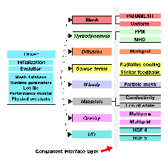
An abstract representation of the FLASH architecture appears in Figure 3. Each box in this figure represents a component (FLASH module), which publishes a small set of public methods to its clients. These public methods are expressed through virtual function definitions (stubs under Fortran 90), which are implemented by real functions supplied by sub-modules. Typically each component represents a different class of solver. For time-dependent problems, the driver uses time-splitting techniques to compose the different solvers. The solvers are divided into different classes on the basis of their ability to be composed in this fashion and upon natural differences in solution method (e.g., hyperbolic solvers for hydrodynamics, elliptic solvers for radiation and gravity, ODE solvers for source etc.).

The adaptive mesh refinement module is treated in the same way as the solvers. The means by which the driver shares data with the solver objects is the primary way in which the architecture affects the overall performance of the code. Choices here, in order of decreasing performance and increasing flexibility, include global memory, argument-passing, and messaging. FLASH 2.0 has eliminated global variable access in favor of a well-defined set of accessor and mutator methods managed by the centralized database module. When done with an eye toward optimization, the effects on performance are tolerable, and the benefits for maintainability and extensibility are significant. This is discussed in greater detail below.

3.2.1  Code infrastructure

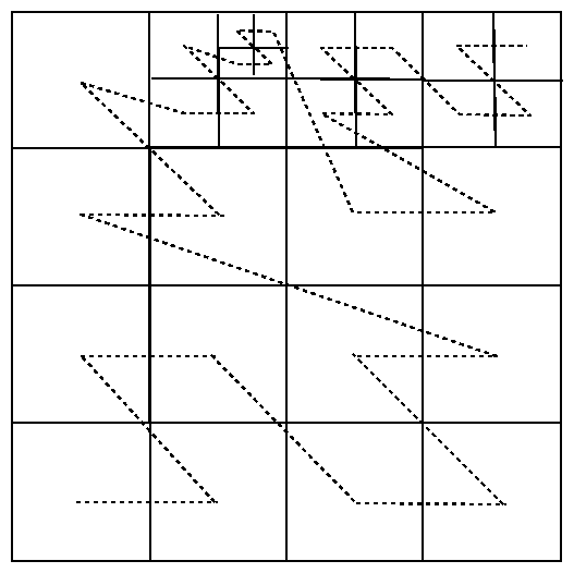
The structure of the FLASH source tree reflects the module structure of the code, as shown in Figure 4 for an older version of FLASH. The general plan is that source code is organized into one set of directories, while the code is built in a separate directory using links to the appropriate source files. The links are created by a source configuration script called setup, which makes the links using options selected by the user and then creates an appropriate makefile in the build directory. The user then builds the executable with a single invocation of gmake.

Source code for each of the different code modules is stored in subdirectories under source/. The code modules implement different physics, such as hydrodynamics, nuclear burning, and gravity, or different major program components, such as the main driver code and the input/output code. Each module directory contains source code files, makefile fragments indicating how to build the module, and a configuration file (see Section 6.1.2).

Each module subdirectory may also have additional sub-module directories underneath it. These contain code, makefiles, and configuration files specific to different variants of the module. For example, the hydro/ module directory can contain files which are generic to hydrodynamical solvers, while its explicit/ subdirectory contains files specific to explicit hydro schemes and its implicit/ subdirectory contains files specific to implicit solvers. Configuration files for other modules which need hydrodynamics can specify hydro as a requirement without mentioning a specific solver; the user can then choose one solver or the other when building the code (via the modules file; Section 6.1.3). When setup configures the source tree it treats each sub-module as inheriting all of the source code, configuration files, and makefiles in its parent module's directory, so generic code does not have to be duplicated. Sub-modules can themselves have sub-modules, so for example one might have hydro/explicit/split/ppm and hydro/implicit/ppm. Source files at a given level of the directory hierarchy override files with the same name at higher levels, whereas makefiles and configuration files are cumulative. This permits modules to supply stub routines that are treated as `virtual functions' to be overridden by specific sub-modules, and it permits sub-module directories to be self-contained.

When a module is not explicitly included by Modules, only one thing is done differently by setup: sub-modules are not included, except for a null sub-module, if it is present. Most top-level modules should contain only stub files to be overridden by sub-modules, so this behavior allows the module to be `not included' without extra machinery (such as the special stub files and makefiles required by earlier versions of FLASH). In those cases in which the module's files are not appropriate for the `not included' case, the null sub-module allows one to override them with appropriate versions.

New solvers and new physics can be added. At the current stage of development of FLASH it is probably best to consult the authors of FLASH (see Section 7) for assistance in this. Some general guidelines for adding solvers to FLASH 2.0 may be found in Section 17.

The setups/ directory has a structure similar to that of source/. In this case, however, each of the "modules" represents a different initial model or problem, and the problems are mutually exclusive; only one is included in the code at a time. Also, the problem directories have no equivalent of sub-modules. A makefile fragment specific to a problem need not be present, but if it is, it is called Makefile. Section 16 describes how to add new problem directories.

The setup script creates a directory called object/ in which the executable is built. In this directory setup creates links to all of the source code files found in the specified module and sub-module directories as well as the specified problem directory. (A source code file has the extension .c, .C, .f, .f90, .F90, .F, .fh, or .h.) Because the problem setup directory and the machine-dependent directory are scanned last, links to files in these directories override the ``defaults'' taken from the source/ tree. Hence special variants of routines needed for a particular problem can be used in place of the standard versions by simply giving the files containing them the same names.

Using information from the configuration files in the specified module and problem directories, setup creates a file named init_global_parms.F90 to parse the runtime parameter file and initialize the runtime parameter database. It also creates a file named rt_parms.txt, which concatenates all of the PARAMETER statements found in the appropriate configuration files and so can be used as a ``master list'' of all of the runtime parameters available to the executable.

setup also creates makefiles in object/ for each of the included modules. Each copy is named Makefile.module, where module is driver, hydro, gravity, and so forth. Each of these files is constructed by concatenating the makefiles found in each included module path. So, for example, including hydro/explicit/split/ppm causes Makefile.hydro to be generated from files named Makefile in hydro/, hydro/explicit/, hydro/explicit/split/, and hydro/explicit/split/ppm/. If the module is not explicitly included, then only hydro/Makefile is used, under the assumption that the subroutines at this level are to be used when the module is not included. The setup script creates a master makefile (Makefile) in object/ which includes all of the different modules' makefile fragments together with the site- or operating system-dependent Makefile.h.

The master Makefile created by setup creates a temporary subroutine, buildstamp.F90, which echoes the date, time, and location of the build to the FLASH log file when FLASH is run. To ensure that this subroutine is regenerated each time the executable is linked, the Makefile deletes buildstamp.F90 immediately after compiling it.

The setup script can be run with the -portable option to create a directory with real files which can be collected together with tar and moved elsewhere for building. In this case the build directory is assigned the name object_problem/. Further information on the options available with setup may be found in Section 13. .

Additional directories included with FLASH are tools/, which contains tools for working with FLASH and its output (Sec:FLASH output comparison utility), and docs/, which contains documentation for FLASH (including this user's guide) and the PARAMESH library.

3.3  Modules included with FLASH: a brief overview

The current FLASH distribution comes with a set of core components that form the backbone of many common problems, namely: database, driver, hydro, io, mesh, particles, source_terms, gravity, and materials. A detailed discussion of the role of each of these modules is presented in Part IV. Here we give a brief overview of each.

Section 4 describes in detail the various driver modules which may be implemented with FLASH. In addition to the default driver, which controls the initialization, evolution, and output of a FLASH simulation, four new driver modules have been written to implement different explicit time advancement algorithms. Three are written in the delta formulation: euler1, rk3, and strang_delta. The fourth, strang_state, is written in the state-vector formulation. A subsection concerning simulation services, runtime parameters, and logfiles is also included in this section.

Section 5 describe the FLASH I/O modules, which control how FLASH data structures are stored on different platforms and in different formats. Discussed in this section are the main I/O module hdf4, which uses the Hierarchical Data Format (HDF) for storing simulation data, two major HDF5 modules (serial and parallel versions), and Fortran 77 (f77) modules.

Section 6 describes the mesh module, together with the PARAMESH package of subroutines for the parallelization and adaptive mesh refinement (AMR) portion of FLASH.

Section 7 describes the two hydrodynamic modules included in FLASH 2.x. The first is based on the PROMETHEUS code (Fryxell, Müller, and Arnett 1989); the second is based on Kurganov numerical methods.

Section 8 describes the magnetohydrodynamics module included with the FLASH code, which solves the equations of ideal MHD.

Section 9 discusses the material properties module, which handles the tracking of multiple fluids in FLASH simulations. It includes the equation of state module, which implements the EOS for the hydrodynamical and nuclear burning solvers; the composition submodule, which sets up the different compositions needed by FLASH; and the stellar conductivity module, which may be used for computing the opacity of stellar material. Section describes source terms, including the nuclear burning module, which calculates the nuclear burning rate of a hydrodynamical simulation, and the stirring module, which adds a divergence-free, time-correlated `stirring' velocity at selected modes in a given hydrodynamical simulation.

Section 11 describes the gravity module, which computes gravitational potential or gravitational acceleration source terms for the code. It includes several sub-modules: the constant submodule, the plane parallel sub-module, the ptmass submodule, and the Poisson submodules.

Part 3
MODULES

4  Driver modules

The driver module controls the initialization, evolution, and output of a FLASH simulation. Initialization can be from scratch or from a stored checkpoint file. Evolution can use any of several different operator-splitting techniques to combine different physics operators and integrate them in time, or call a single operator if the problem of interest is not time-dependent. Output involves the production of checkpoint files, plot files, analysis data, and log file time stamps. In addition to these functions, the driver supplies important simulation services to the rest of the FLASH framework, including Fortran modules to handle runtime parameters, physical constants, memory usage reports, and log file management (these are discussed further in Section ).

The initialization and termination routines and simulation services modules are common to both time-dependent and time-independent drivers and thus are included at the highest level of driver. The file flash.F90 contains the main FLASH program (equivalent to main() in C) and calls these routines as needed. The default flash.F90 is empty and is intended to be overridden by submodules of driver. At this time only time-dependent drivers are supplied with FLASH; these are submodules of the driver/time_dep module. The time_dep version of flash.F90 calls the FLASH initialization routine, loops over timesteps, and then calls the FLASH termination routine. During the time loop it computes new timesteps, calls an evolution routine (evolve()), and calls output routines as necessary.

The details of each available time integration method are completely determined by the version of evolve() supplied by that method. The default time update method is to call each physics module's update routine for two equal timesteps - thus, hydro, source terms, gravity, hydro, source terms, gravity. The hydrodynamics update routines take a ``sweep order'' argument in case they are directionally split; in this case, the first call uses the ordering x-y-z, and the second call uses z-y-x. Each of the update routines is assumed to directly modify the solution variables. At the end of each pair of timesteps, the condition for updating the mesh refinement pattern is tested, and a refinement update is carried out if required.

The alternative ``delta formulation'' drivers (driver/time_dep/delta_form) modify a set of variables containing the change in the solution during the timestep. The change is only applied to the solution variables after all operators have been invoked. This technique permits more general time integration methods, such as Runge-Kutta methods, to be employed, and it provides a more flexible method for composing operators. However, only a few physics modules can make use of it as yet. More details on the delta formulation drivers appear in Section 4.1.

The driver module supplies certain runtime parameters regardless of which type of driver is chosen. These are described in Table 1.

4.1  New driver modules euler1, rk3, and strang_delta

New driver modules have been written to implement different explicit time advancement algorithms. This usage of the driver modules is slightly different than that of the default driver module, which does not directly implement a time advancement algorithm; the default driver and hydro modules each implement parts of the Strang splitting time advancement. First, a listing of the time advancement tasks common to all of the new drivers will be given. In following subsections, the details of each time advancement method will be described.

The three driver modules written in the delta formulation are euler1, rk3, and strang_delta. They make appropriate calls to the physics modules, and update the solution by calling functions provided by the formulation module. The strang_state driver is written in the state-vector formulation; it also calls the physics modules, but does not update the solution. To use the new modules, first choose the driver by including one of the following lines into the Modules file.

/driver/time_dep/delta_form/euler1
/driver/time_dep/delta_form/rk3
/driver/time_dep/delta_form/strang_delta
/driver/time_dep/delta_form/strang_state

/formulation/delta_form

/formulation

For delta formulation time advancements, the new driver modules use the formulation module to hold and access the global DU array, and to update the solution. In the state-vector formulation, the formulation module is not directly used by the driver; instead, the physics modules call the update subroutines the formulation module provides.

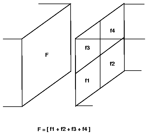
The new driver modules discretize the left-hand side of

¶V ¶t = (spatial difference terms)+ (source terms).

(3)

The time advancement algorithm is contained in a subroutine named evolve. Each call to evolve advances the solution through one time step, Dt. Each time advancement algorithm begins with a vector of primary variables, Vⁿ at time tⁿ, and an associated set of auxiliary variables, Wⁿ. Primarily through calls to other physics modules, evolve applies a set of operations to the variables to produce an updated vector, Vⁿ⁺¹ at time t_n+1 = t_n + Dt. Depending on the formulation, the time advancement may or may not update the auxiliary variables - in the state-vector formulation, the other physics modules update them.

The distinction between V and W is that time-dependent differential equations are solved to determine the primary variables. The auxiliary variables are obtained from the primary variables through algebraic relations. Often the primary variables are the conserved variables, U, and in the rest of this section U will replace V. However, the time advancement algorithms implemented do not require this correspondence.

The time advancement algorithms are written generally, in that each differential equation is treated in the same way. The distinction between the equations (for example, between the x-momentum equation and the total energy equation) is expressed in the other physics modules. The time advancement algorithm does not need to know the identity of the variables on which it operates, except possibly to update the auxiliary variables from the primary variables; but this update is handled by a call to a subroutine provided by the formulation module.

4.1.1  The euler1 module

The euler1 module implements the first-order, Euler explicit scheme:

Un+1 = Un + Dt L(Un)

(4)

where L(U) represents all of the physics modules. The euler explicit method is implemented in the delta formulation. No runtime parameters are defined for this module.

At the beginning of a time step, DU is set to zero. Each of the physics modules is called, with Uⁿ as the initial state, and adds its contribution to DU. After all the physics modules have been called, the global DU array holds L(Uⁿ). Equation (4) yields Uⁿ⁺¹. Finally, the auxiliary variables are updated from the conserved variables with a call to the global update subroutine provided by the formulation module.

Note that because all the physics modules start with the same initial state, the order in which the physics modules are called does not affect the results (except possibly through floating point roundoff differences when contributing to DU.)

The set of steps, consisting of calls to physics modules, updating the conserved variables, and updating the auxiliary variables, is often called a stage. The majority of the computational cost of a stage is the in the calls to the other physics modules; this component corresponds to a ``function evaluation'' for ordinary differential equation solvers. In the Euler explicit algorithm, there is one stage per time step.

4.1.2  The rk3 module

Runge-Kutta schemes are a class ordinary differential equation solvers which are appreciated for their higher order of accuracy, ease of implementation, and relatively low storage requirements. There are many third-order Runge-Kutta methods; all require at least three stages. Most require at least three storage locations per primary variable, but the one implemented in the delta formulation in FLASH, derived by Williamson (J. Comp. Phys. 35:48, 1980) requires only two.

The two storage registers will be referred to as U and DU. The global solution vector, U, holds Uⁿ at the beginning of the time step, then intermediate solutions U^(·) at the end of each stage. The manipulation of the global DU array is more complicated. DU accumulates contributions from the physics modules during a stage, but it also holds results from previous stages; it is important to distinguish between the results of the physics modules, L(U), and the quantity held in the global DU array. First the algorithm will be shown; then the usage of the global DU array will be discussed. For the equation

¶U ¶t = L(U),

(5)

Williamson's algorithm is, starting with Uⁿ,

U(1) = Un +  1 3 Dt é ë L(Un) ù û (6) U(2) = U(1) +  15 16 Dt é ë L(U(1)) -  5 9 L(Un) ù û (7) Un+1 = U(3) = U(2) +  8 15 Dt é ë L(U(2)) -  153 128 æ è L(U(1)) -  5 9 L(Un) ö ø ù û . (8)

U^(m) is the result of the m-th stage, and the auxiliary variables are updated each time a new U^(m) is computed.

The algorithm is implemented using the following steps to attain the low storage. At the beginning of the time step, DU is set to zero. During the first stage each physics module contributes to DU, so after all have contributed, DU holds the bracketed term in eq. (6), L(Uⁿ). U⁽¹⁾ is then computed using eq. (6). Stage 1 is completed by multiplying DU by -5/9, which is required for the following stages. The process is repeated for stage 2: after the physics modules have contributed, DU holds the bracketed term in eq. (7); U⁽²⁾ is computed by eq. (7) and stored in U; then DU is multiplied by -153/128. Stage 3 is similar, but ends after U⁽³⁾ = Uⁿ⁺¹ is computed and stored. It is critical that the only changes made to the DU array are those just listed; no physics module should change the value of DU, except to add its contribution, and since DU holds information from previous stages, it should not be reset to zero except at the beginning of the time step.

No runtime parameters are defined for this module.

4.1.3  strang_state and strang_delta modules

The second-order accurate splitting method (Strang 1968) is attractive because of its low memory requirements. The algorithm is based on the operator splitting approach, in which a set of subproblems is solved rather a single complicated problem. Each subproblem typically accounts for one term in a system of partial differential equations, representing a particular type of physics and for which an appropriate (specialized) numerical method is available. The basic operator splitting method is first-order accurate, but the Strang splitting scheme is second-order accurate over two time steps. In the first time step, the subproblems are solved in a given sequence. Second-order accuracy is obtained by reversing the sequence in the second time step.

A key feature of the operator splitting approach is that the output of one subproblem is the input to the next subproblem. This allows an implementation that, globally, stores only the current solution, but can also cause problems including accuracy losses due to decoupling various physical effects (splitting errors) and difficulties implementing boundary conditions.

In practice it has been found that splitting errors are reduced when the subproblems are ordered in increasing stiffness, i.e. the stiffest subproblem is solved last in the sequence; this has recently been supported by numerical analysis (Sportisse 2000).

Two new driver modules implement an algorithm similar to the Strang splitting time advancement. Since the sequence is not exactly reversed in the second step compared to the first, the algorithm is not the true Strang splitting. However, the source terms include nuclear burning source terms which are very stiff, and there are sound arguments for computing them last. The strang_state module implements the algorithm in the state-vector formulation, and is recommended for ``production'' runs for its low memory requirements. The strang_delta driver is implemented in the delta formulation and is provided for testing and comparison. For both versions, one call to evolve (which implements the time advancement algorithm) advances the solution from tⁿ to tⁿ⁺², i.e. over two time steps.

In the strang_state driver, the sequence of calls to physics modules in the first time step is

hydro(x-sweep)
hydro(y-sweep)
hydro(z-sweep)
gravity
source terms

hydro(z-sweep)
hydro(y-sweep)
hydro(x-sweep)
gravity
source terms

No runtime parameters are defined for either module.

4.1.3.1  New formulation modules  

The purposes of this module class are

1. To provide functions, usable by physics modules and driver modules,

   to update the solution locally (on a block or a face of a block) or globally (on all blocks.)

2. If needed by the time advancement (driver) module, to provide storage space for the global DU array and functions to access it.

The services provided to delta formulation drivers are a superset of those provided to drivers in the state-vector formulation, and the directory structure is used to express that. The /formulation directory contains the local update subroutines and a version of formulation_Module suitable for the state-vector instantiation. formulation_Module defines a module in the Fortran90 sense, as opposed to the FLASH hierarchy sense. The /formulation/delta_form directory contains the global update subroutine and the version of formulation_Module required for the delta instantiation.

When /formulation is specified in the Modules file, the local update functions and the first formulation_Module are built into the executable, as appropriate for drivers in the state-vector formulation; when /formulation/delta_form is specified in the Modules file, the local update functions, the global update function, and the second version of formulation_Module are used in the executable as required by drivers in the delta formulation. This use of the FLASH code framework and directory hierarchy allows static allocation of the global DU array when needed but saves that memory when not. At the same time it allows local update functions to be used by both state-vector and delta formulations without duplicating code.

Currently the update functions apply only to the particular variable sets described. The local update functions must be given the (old) conserved variables in the order r₁, ¼,r_ionmax, ru, rv, rw, rE, and they store in the database X₁, ¼, X_ionmax, r, P, T, g, u, v, w, and E. The mapping from the conserved variables to the database variables is not general, it is specific to the variables just listed. Variables other than those specifically listed will not be updated, and their influence on the variables just listed will be ignored. Development of more flexible update routines is underway. However, changes will most likely be internal to the local and global update functions, and the organization of these modules is not expected to change.

   4.1.3.1.1  State-Vector Instantiation  

In this subsection the local update functions, named du_update_block, du_update_xface, du_update_yface, and du_update_zface, are described. These subroutines accept local arrays of conserved variables and their changes as inputs, compute updated conserved variables, compute auxiliary variables from algebraic relations (with the aid of appropriate equation of state calls), and store the updated variables in the database.

These subroutines accept the block number, a local DU, local conserved variables U, the time step Dt, and a scalar factor c, all as passed arguments. The face update routines also accept an index specifying which grid plane to update. The conserved variables are those listed in eq.(). The conserved variables are updated by

Unew = Uold + c Dt DU.

(9)

The factor c allows an update to an intermediate time between tⁿ and tⁿ⁺¹, often required by Runge-Kutta time advancement methods; it is intended for use by drivers in the delta formulation through the global update subroutine.

From the updated conserved variables, all variables stored in the database are computed. The density, r, and species mass fractions, X_s, are obtained from the species densities, r_s. The velocity components u, v, and w and the total energy per unit volume E are computed from the momenta and total energy per unit mass, respectively, by dividing by r. The internal energy, e_i, is calculated by subtracting the kinetic energy, (u² + v² +w²)/2, from E. The temperature, T, pressure, P, and ratio of specific heats, g are obtained through a call to the equation of state, for which r, X_s, and e_i are inputs.

Finally, the updated variables are stored in the variable database. The variables stored are X_s, r, P, T, g, u, v, w, and E. Only the interior cells of a block or face are updated; for all guard cells, zeros are stored for all updated variables. None of the calculations described above are executed for the guard cells.

For the state-vector formulation, there are only a few tasks for the Fortran 90 module formulation_Module. First, it defines a Fortran logical parameter delta_formulation to be `false'. This parameter is designed to be accessed by physics modules. When false, it indicates that each physics module should update the solution; while the local update routines just described are recommended for this purpose, there is no requirement that they be used. Second, formulation_Module defines several parameters for sizing arrays and a set of integers (indices) used to access the variable database; these are used by the local update subroutines.

In the state-vector instantiation, formulation_Module does not declare the global DU array. It does define some functions which are used to access that array, but in this instantiation they do not perform any operations - they are `stub' functions. The reason for defining them is as follows. If a physics module is written so that either the state-vector or delta formulation can be used, it must include calls to functions which access the global DU array. When the state-vector formulation is used these calls are not made, but some compilers might raise errors if these functions were not defined. By defining them in this instantiation of formulation_Module, such errors are avoided. The stub functions are contained, in the Fortran 90 sense, in formulation_Module. The local update functions are not contained in the formulation_Module, although they directly access the array sizing parameters and database indices therein.

   4.1.3.1.2  Delta Instantiation  

In this section the global update subroutine du_update and the delta formulation version of formulation_Module are described. The global update routine is a wrapper to the local update subroutine du_update_block. Two arguments, c and Dt, are passed into du_update. For each block, it gets r, X_s, u, v, w, and E from the database; computes the (old) conserved variables from these; gets the DU for the block from the global DU array; and calls du_update_block. Recall that du_update_block computes the updated variables and stores them in the database.

For the delta instantiation, formulation_Module defines the same array-sizing parameters and database indices as in the state-vector instantiation. However, it defines the parameter delta_formulation to be `true', indicating to the physics modules that their contributions should be added to the global DU array. The delta instantiation of formulation_Module statically allocates the global DU array, and defines several functions to manipulate it. Each element of the global DU array is set to zero by du_zero. A physics module can add its local DU for a block to the global array by calling du_block_to_global; the subroutines du_xface_to_global, du_yface_to_global and du_zface_to_global do the same for faces (slices) of a block. These subroutines are contained in formulation_Module, and are the actual, working versions of the stub functions defined in the state-vector instantiation.

The global DU array is a public, module-scope variable in the Fortran 90 sense. The du_update subroutine is not contained in formulation_Module, but can access the array-sizing parameters and database indices in the module. It can also access the global DU array directly, and is the only subroutine not contained in formulation_Module allowed to do so.

4.2  Simulation services

4.2.1  Runtime parameters

The driver module provides a Fortran 90 module called runtime_parameters. The routines in this module maintain `parameter contexts,' essentially small databases of runtime parameters. Contexts can be created and destroyed, and runtime parameters can be added to them, have their values modified, and be queried as to their value or data type. These features allow a program to maintain several contexts for different code modules without having to declare and share the parameters explicitly. User-written subroutines (e.g., for initialization) should use the routines in this module to access the values of any runtime parameters they require.

An example of the application of this module is to use the read_parameters() routine (separately supplied) to parse a text-format input file containing parameter settings. The calling program declares a context, adds parameters to it, then calls read_parameters() to parse the input file. Finally, the context is queried to obtain the input values. Such a program might look like the following code fragment.

	program test
	use runtime_parameters
	type (parm_context_type) :: context
	real			 :: x_init
	...
	call create_parm_context (context)
	call add_parm_to_context (context, "x_init", 4.)
	...
	call read_parameters ("input.par", context)
	call get_parm_from_context (context, "x_init", x_init)
	...
	end

	integer n_x
	call add_parm_to_context (context, "N_x", 32)
	call get_parm_from_context (context, "n_X", n_x)
	write (*,*) n_x
	call set_parm_in_context (context, "n_x", 64)
	call get_parm_from_context (context, "N_X", n_x)
	write (*,*) n_x

	32
	64

The following routines, data types, and public constants are provided by this module. Note that the main FLASH initialization routine (init_flash()) and the initialization code created by setup already handle the creation of the database and the parsing of the parameter file, so users will mainly be interested in querying the database for parameter values.

• parm_context_type

  Data type for contexts.

• global_parm_context

  A parameter context available to all program units which use the runtime_parameters module. This is made available only for programs which share the rest of their data among routines via included common blocks. Programs which use modules should declare their own contexts within their modules.

• parm_{real,int,str,log,invalid}

  Constants returned by get_parm_type_from_context().

• create_parm_context (c)

  Create context c.

• destroy_parm_context (c)

  Destroy context c, freeing up the memory occupied by its database.

• add_parm_to_context (c,p,v)

  Add a parameter named p to context c. p is a character string naming the parameter, and v is the default or initial value to assign to the parameter. v can be of type real, integer, string, or logical. The type of v sets the type of the parameter; subsequent sets or gets of the parameter must be of the same type, or an error message will be printed.

• set_parm_in_context (c,p,v)

  Set the value of parameter p in context c equal to v. p is a character string naming the parameter, which must already have been created by add_parm_to_context (else an error message is printed). The type of v must match the type of the initial value used to create the parameter, else an error message is printed.

• get_parm_from_context (c,p,v)

  Query context c for the value of parameter p and return this value in the variable v. Parameter p must already exist, and the type of v must match the type of the initial value used to create the parameter, else an error message is printed.

• get_parm_type_from_context (c,p,t)

  Query context c for the data type of parameter p. The result is returned in t, which must be of type integer. Possible return values are parm_real, parm_int, parm_str, parm_log, and parm_invalid. parm_invalid is returned if the named parameter does not exist.

• list_parm_context (c,l)

  Print (to I/O unit l) the names and values of all parameters associated with context c.

• bcast_parm_context (c,p,r)

  Broadcast the parameter names and values from a specified context c to all processors. p is the calling processor's rank, and r is the rank of the root processor (the one doing the broadcasting).

4.2.2  Physical constants

The driver supplies a Fortran 90 module called physical_constants, which maintains a centralized database of physical constants. The database can be queried by string name and optionally converted to any chosen system of units. The default system of units is CGS. This facility makes it easy to ensure that all parts of the code are using a consistent set of physical constant values and unit conversions and to update the constants used by the code as improved measurements become available.

For example, a program using this module might obtain the value of Newton's gravitational constant G in units of Mpc³ Gyr^-2 M_\odot^-1 by calling

	call get_constant_from_db ("Newton", G, len_unit="Mpc",
			     time_unit="Gyr", mass_unit="Msun")

Physical constants are taken from the 1998 Review of Particle Properties, Eur. Phys. J. C 3, 1 (1998), which in turn takes most of its values from Cohen, E. R. and Taylor, B. N., Rev. Mod. Phys. 59, 1121 (1987). The following routines are supplied by this module.

• get_constant_from_db (n,v[,units])

  Return the value of the physical constant named n in the variable v. Optional unit specifications are used to convert the result. If the constant name or one or more unit names aren't recognized, a value of 0 is returned.

• add_constant_to_db (n,v,len,time,mass,temp,chg)

  Add a physical constant to the database. n is the name to assign, and v is the value in CGS units. len, time, mass, temp, and chg are the exponents of the various base units used in defining the unit scaling of the constant. For example, a constant with units (in CGS) of cm³ s^-2 g^-1 would have len=3, time=-2, mass=-1, temp=0, and chg=0.

• add_unit_to_db (t,n,v)

  Add a unit of measurement to the database. t is the type of unit (``length,'' ``time,'' ``mass,'' ``charge,'' ``temperature''), n is the name of the unit, and v is its value in terms of the corresponding CGS unit. Compound units are not supported, but they can be created as physical constants.

• init_constants_db ()

  Initialize the constants and units databases. Can be called by the user program, but doesn't have to be, as it is automatically called when needed (ie. if a ``get'' or ``add'' is called before initialization).

• list_constants_db (lun)

  List the constants and units databases to the specified logical I/O unit.

• destroy_constants_db ()

  Deallocate the memory used by the constants and units databases, requiring another initialization call before they can be accessed again.

4.2.3  Monitoring performance

FLASH includes a set of routines for monitoring performance. The routines start or stop a timer at the beginning or end of the routine(s) to be monitored and accumulate time in dynamically assigned accounting segments. At the completion of the program, the routines write out a performance summary. We note that these routines are not recommended for use in timing very short segments of code due to the overhead in accounting.

All of the source code for the performance monitoring can be found in the module file perfmon.F90. The list below contains the performance routines along with a short description of each. Many of the subroutines are overloaded to take either a module name or an integer index.

• timer_init ()

  Initializes the performance accounting database. Calls system time routines to subtract out their initialization overhead.

• timer_create (module,id)

  Creates a timer and returns a unique integer index for the timer.

• timer_start(module)

  Subroutine that begins monitoring code module module or module associated with index id. If module is not associated with a previously assigned accounting segment, the routine creates one, whereas if id is not associated with one, then nothing is done. The parameter module is specified with a string (max 30 characters). Calling timer_start on the same module more than once without first calling timer_stop causes the current timer for that module to be reset (the accumulated time in the corresponding accounting segment is not reset). Timing modules may be nested as many times as there are slots for accounting segments (see MaxModules setting). Routine may be called with an integer index in addition to the name of the module.

• timer_stop(module)

  Stops accumulating time in the accounting segment associated with code module module. If timer_stop is called for a module which does not exist or for a module which is not currently being timed, nothing happens. Routine may be called with an integer index in addition to the name of the module.

• timer_value(module)

  Returns the current value of the timer for the accounting segment associated with the code module module or referenced by index id. If timer_value is called for a module which does not exist, 0. is returned.

• timer_reset(module)

  Resets the accumulated time in the accounting segment corresponding to the specified code module. Routine may be called with an integer index in addition to the name of the module.

• timer_lookup_index(module)

  Function that given a string module name returns an integer index. The integer index can be used in any of the overloaded timer routines. If a timer name is not found, the function returns timer_invalid. Use of this function to obtain an integer index and subsequently calling the routines by that index rather than the string name is encouraged for performance reasons.

• perf_summary (lun, n_period)

  Subroutine that writes a performance summary of all current accounting segments to the file associated with logical unit number lun. Included is the average over n_period intervals (eg. timesteps). The accounting database is not reinitialized. lun and n_period are of default integer type. Calling perf_summary stops all currently running timers.

Below is a very simple example of calling the performance routines.

       program example
       integer i
       call timer_init
       do i = 1, 1000
         call timer_start ('blorg')
         call blorg
         call timer_stop ('blorg')
         call timer_start ('gloob')
         call gloob
         call timer_stop ('gloob')
       enddo
       call perf_summary (6, 1000)
       end

4.2.4  Log file maintenance

The driver supplies a Fortran 90 module called logfile to manage the FLASH log file, which contains various types of useful information, warnings, and error messages produced by a FLASH run. User-written routines may also make use of this module as needed. The logfile routines enable a program to open and close a log file, write time or date stamps to the file, and write arbitrary messages to the file. The file is kept closed and is only opened for appending when information is to be written, avoiding problems with unflushed buffers. For this reason, logfile routines should not be called within time-sensitive loops, as the routines will generate system calls.

An example program using the logfile module might appear as follows:

	program test
	use logfile
	integer :: i
	call create_logfile ("test.log",  "test.par", .false.)
	call stamp_logfile ("beginning log file test...")
	do i = 1, 10
	  call open_logfile
	  write (log_lun,*) 'i = ', i
	  call close_logfile
	enddo
	call stamp_logfile ("done with log file test.")
	end

• create_logfile (name, parmfile, restart)

  Creates the named log file and writes some header information to it, including the build stamp and the values of all runtime parameters in the global parameter context. The name of the parameter file is taken as an input; it is echoed to the log file. If restart is .true., the file is opened in append mode.

• stamp_logfile (string)

  Write a date stamp and a specified string to the log file.

• tstamp_logfile (n, t, dt)

  Write a dated timestep stamp for step n, time t, timestep dt to the log file. n must be an integer, while t and dt must be reals.

• write_logfile (string)

  Write a string to the log file without a date stamp.

• break_logfile()

  Write a `break' (a row of ) to the log file.

• open_logfile()

  Open the log file for writing, creating it first with a default name (logfile) if necessary. open_logfile() and close_logfile() should only be used if it is necessary to write something directly to the log file unit with some external routine.

• close_logfile()

  Close the log file.

• log_lun

  The logical unit number being used by the logfile module (to permit direct writes to the log file by external routines).

5  FLASH I/O modules and output formats

Currently FLASH can store simulation data in three basic output formats: Fortran 77 binary, Hierarchical Data Format (HDF) (sometimes called HDF 4), and HDF5. In general, these format are not compatible, but some tools for translating from one format to the other exist. These formats control how the binary data is stored on disk, how to address it, what to do about different data storage on different platforms. The mapping of FLASH data-structures to records in these files is controlled by the FLASH I/O modules. These file formats have different strengths and weaknesses, and the data layout is different for each file type.

Different techniques can be used to write the data to disk: move all the data to a single processor for output; have each processor write to a separate file; and parallel access to a single file. In general, parallel access to a single file will provide the best performance. On some platforms, such as Linux clusters, there may not be a parallel filesystem, so moving all the data to a single process is the best solution.

The default I/O module in FLASH is hdf4, which uses the HDF format. The HDF format provides an application programming interface (API) for organizing data in a database fashion. In addition to the raw data, information about the data type and byte ordering (little or big endian), rank, and dimensions of the dataset is stored. This makes the HDF format extremely portable across platforms. Different packages can query the file for its contents, without knowing the details of the routine that generated the data.

HDF is limited to files < 2 GB is size. Furthermore, the official release of HDF does not support parallel I/O. To address these limitations, HDF5 was released. HDF5 is supported on a large variety of platforms, and offers the same functionality as HDF, with the addition of large file support and parallel I/O via MPI-I/O. Information of the different versions of HDF can be found at http://hdf.nsca.uiuc.edu. This section assumes that you already have the necessary HDF libraries installed on your machine.

The I/O modules in FLASH have two responsibilities-generating and restarting from checkpoint files, and generating plot files. A checkpoint file contains all the information needed to restart the simulation. The data is stored at the same precision (8-byte reals) as it is carried in the code, and includes all of the variables. A plotfile contains all the information needed to interpret the tree structure maintained by FLASH and it contains a user-defined subset of the variables. Furthermore, the data may be stored at reduced precision to conserve space.

The type of output you create will depend on what type of machine you are running on, the size of the resulting dataset, and what you plan on doing with the datafiles once created. Table 2 summarizes the different modules which come with FLASH 2.0.

It is strongly recommended that you use one of the HDF5 output formats with FLASH. These are currently the best performing I/O modules in FLASH. Furthermore, support for HDF5 exists for just about every platform you are likely to encounter.

5.1  General parameters

There are several parameters that control the frequency of output, type of output, and name of the output files. These parameters are the same for all the different modules, although not every module is required to implement all parameters. Some of these parameters are used in the top level I/O routines (initout.F90, output.F90, and finalout.F90) to determine when to output, while others are used to determine the resulting filename. Table 3 gives a description of the I/O parameters.

Table 5: General I/O parameters.
Parameter	Type	Default value	Description
Table 6: FLASH I/O parameters (continued).
Parameter	Type	Default value	Description
rolling_checkpoint	INTEGER	10000	The number of checkpoint files to keep available at any point in the simulation. If a checkpoint number is > rolling_checkpoint, then the checkpoint number is reset to 0. There will be at most rolling_checkpoint checkpoint files kept. This parameter is intended to be used when disk space is at a premium.
wall_clock_checkpoint	REAL	43200	The maximum amount of wall clock time to go between checkpoints. When the simulation is started, the current time is stored. If wall_clock_checkpoint seconds elapse over the course of the simulation, a checkpoint file is stored. This is useful to ensure that a checkpoint file is produced before a queue closes.
basenm	STRING	``chkpnt''	The main part of the output filenames. The full filename consists of the basename a series of three character abbreviations indicating whether it is a plotfile or checkpoint file, and the format, and a 4-digit file number. See § 5.1.1 for a description of how FLASH output files are named.
cpnumber	INTEGER	10000	The number of the current checkpoint file. This number is appended to the end of the basename when creating the filename. When restarting a simulation, this indicates which checkpoint file to use.
ptnumber	INTEGER	1	The number of the current plotfile. This number is appended to the end of the basename when creating the filename.
restart	BOOLEAN	.false.	A logical variable indicating whether the simulation is restarting from a checkpoint file (.TRUE.) or starting from scratch (.FALSE.).
nrstrt	INTEGER	10000	The number of timesteps desired between subsequent checkpoint files.
trstrt	REAL	1	The amount of simulation time desired between subsequent checkpoint files.
tplot	REAL	1	The amount of simulation time desired between subsequent plotfiles.
corners	BOOLEAN	.false.	A logical variable indicating whether to interpolate the data to cell corners before outputting. This only applies to plotfiles.
plot_var_1, ... plot_var_8	STRING	``none''	Name of the variables to store in a plotfile. Up to 8 variables can be selected for storage, and the standard 4-character variable name can be used to select them.

5.1.1  Output file names

FLASH constructs the output filenames based on the user-supplied basename and the file counter that is incremented after each output. Additionally, information about the file type and data storage is included in the filename.
 
The general checkpoint filename is:
basename_{

hdf

hdf5

f77

}_chk_0000,
where hdf, hdf5, or f77 is picked depending on the I/O module used and the number at the end of the filename is the current cpnumber.
 
The general plotfile filename is:
basename_{

hdf

hdf5

f77

}_plt_{

crn

cnt

}_0000,
where hdf, hdf5, or f77 is picked depending on the I/O module used, crn and cnt indicate data stored at the cell corners or centers respectively, and the number at the end of the filename is the current ptnumber.

5.2  Restarting a simulation

In a typical production run, your simulation can be interupted for a number of reasons-machine crashes, the present queue window closes, the machine runs out of disk space, or (*gasp*) a bug in FLASH. Once the problem is fixed, you do not want to start over from the beginning of the simulation, but rather would like to pick up where you left off.

FLASH is capable of restarting from any of the checkpoint files it produces. You will want to make sure the file you wish to restart from is valid (i.e. the code did not stop while outputting). To tell FLASH to restart, set the restart runtime paramter to .TRUE. in your flash.par. You will also want to set cpnumber to the number of the file you wish to restart from. Finally, if you are producing plotfiles, you will want to set ptnumber to the number of the next plotfile you want FLASH to output. Sometimes several plotfiles may be produced after the last valid checkpoint file, so resetting ptnumber to the first plotfile produced after the checkpoint you are restarting from will ensure that there are no gaps in your output.

5.3  Output formats

5.3.1  HDF

The HDF module writes the data to disk using the HDF 4.x library. This module should be supported with HDF 4.1r2 or later. A single file containing the data on all processors is created, if the total size of the dataset is < 2 GB. If there is more than 2 GB of data to be written, multiple files are created to store the data. The number of files used to store the dataset is contained in the number of files record. Each file contains a subset of the blocks (stored in the local blocks record) out of the total number of blocks in the simulation. The blocks are divided along processor boundaries.

The HDF module performs serial I/O-each processors' data is moved to the master processor to be written to disk. This has the advantage of producing a single file for the entire simulation, but is less efficient than if each processor wrote to disk directly. The plotfiles produced with the HDF module contain double precision data. Support for corner data is available with this module.

 
Machine Compatibility

HDF has been tested successfully on most machines, with the exception of (ASC) Red. The HDF library will properly handle different byte orderings across platforms. The IDL tools provided with FLASH will read the FLASH HDF data.

 
Data Format

Table 4 summarizes the records stored in a FLASH HDF file. The format of the plotfiles and checkpoint files are the same, with the only difference being the number of unknowns stored. The records contained in a HDF file can be found via the hdp command that is part of the HDF distribution. The syntax is hdp dumpsds -h filename. The contents of a record can be output by hdp dumpsds -i N filename, where N is the index of the record.

As described above, HDF cannot produce files > 2 GB in size. This is overcome in the FLASH HDF module by splitting the dataset into multiple files when it would otherwise produce a file larger than 2 GB in size.

When reading a single unknown from a FLASH HDF file, you will suffer performance penalties, as there will be many non-unit-stride accesses on the first dimension, since all the variables are stored together in the file.

Table 7: FLASH HDF file format.
Record label	Description of the record
Table 8: HDF 4 format (continued).
Record label	Description of the record
file creation time	character*40 file_creation_time
	The time and date that the file was created.
FLASH version	character*20 flash_version
	This record contains the complete version number of the FLASH distribution you are running. The format is FLASH 2.0.YYYYMMDD where YYYYMMMMDDD is the date of the release. This data is contained in the file RELEASE and the version number is obtained from the flash_release function.
run comment	character*80 run_comment
	The run_comment that was defined for the present simulation. This is a runtime parameter that is useful for notating a simulation.
total blocks	integer tot_blocks
	The total number of blocks in the simulation.
	Note: the number of blocks contained in this file may be less than the total number of blocks if the output is spread across multiple files (see `number of files' and `local blocks')
time	real time
	The simulation time at file output.
timestep	real dt
	The current timestep.
number of steps	integer nsteps
	The number of timesteps from the start of the calculation.
number of blocks per zone	real nblocks_per_zone(3)
	The number of zones in each direction:
	nblocks_per_zone(1) - x-direction
	nblocks_per_zone(2) - y-direction
	nblocks_per_zone(3) - z-direction
number of files	integer num_files
	The number of files that the dataset comprises. Because the filesize cannot be larger than 2 GB, the data is split into multiple files if necessary, with each containing roughly the same number of blocks.
local blocks	integer local_blocks
	The number of blocks in this file. If there are multiple files, this number will be less than `total blocks'.
unknown names	character*4 unk_names(nvar)
	This array contains 4 character names corresponding to the first index of the unk array. They serve to identify the variables stored in the `unknowns' record.
refine level	integer lrefine(local_blocks)
	This array stores the refinement level for each block.
node type	integer nodetype(local_blocks)
	This array stores the nodetype for a block. Blocks with nodetype = 1 are leaf nodes, and this data will always be valid. For plotting purposes, it is the leaf data that you want to plot.
gid	integer gid(nfaces+1+nchild,local_blocks)
	This is the global identification array. For a given block, this array gives the block number of the blocks that neighbor it, and the block number of its parent and children.
	The first nfaces elements point to the neighbors (at the same level of refinement). The faces are numbered from minimum to maximum coordinate with x first, followed by y, and z. A -1 indicates that there is no neighbor at the same level of refinement. A number < = -20 indicates that you are on the physical boundary of the domain. If the neighbor points to the current block, it means that there are periodic boundary conditions. The next element points to the parent of the current block, and the last nchild elements point to the children of the current block.
	Ex: below is a simple domain, assume that at the boundaries, everything is -20
	looking at block no 5 (2-d):
	gid(1,block_no) = 4
	gid(2,block_no) = -1
	gid(3,block_no) = 3
	gid(4,block_no) = -20
	gid(5,block_no) = 1   (the parent)
	gid(6,block_no) = -1  (the children)
	gid(7,block_no) = -1
	gid(8,block_no) = -1
	gid(9,block_no) = -1
	looking at block no 1:
	gid(1,block_no) = -20
	gid(2,block_no) = 6
	gid(3,block_no) = -20
	gid(4,block_no) = -20
	gid(5,block_no) = -1
	gid(6,block_no) = 2
	gid(7,block_no) = 3
	gid(8,block_no) = 4
	gid(9,block_no) = 5
coordinates	real coord(ndim,local_blocks)
	This array stores the coordinates of the center of the block.
	coord(1,block_no) = x-coordinate
	coord(2,block_no) = y-coordinate
	coord(3,block_no) = z-coordinate
block size	real size(ndim,local_blocks)
	This array stores the dimensions of the current block.
	size(1,block_no) = x size
	size(2,block_no) = y size
	size(3,block_no) = z size
bounding box minimum	real bnd_box_min(ndim,local_blocks)
	This array stores the coordinate of the minimum block edge in each direction.
	bnd_box_min(1,block_no) = minimum x edge
	bnd_box_min(2,block_no) = minimum y edge
	bnd_box_min(3,block_no) = minimum z edge
bounding box maximum	as above, but the maximum edge value in each direction.
processor number	integer proc_num(local_blocks)
	The processor number that each block was stored on. This is not used by FLASH, but is useful for debugging purposes, to look at the domain decomposition.
unknowns	real unk(nvar,nx,ny,nz,local_blocks)
	nx = no. of zones/block in x
	ny = no. of zones/block in y
	nz = no. of zones/block in z
	This array holds the unknowns. The variables corresponding to the first argument are listed in the `unknown names' record. Note, for a plot file with CORNERS=.TRUE. in the parameter file, the information is interpolated to the zone corners before being stored. This is useful for certain plotting packages.

5.3.2  HDF5

There are two major HDF5 modules, the serial and parallel version. The format of the output file produced by these modules is identical; only the method by which it is written differs. It is possible to create a checkpoint file with the parallel routines and restart FLASH from that file using the serial routines. In each module, the plot data are written out in single precision to conserve space. These modules require HDF5 1.4.0 or later. At the time of this writing, the current version of HDF5 is 1.4.1.

5.3.2.1  Machine Compatibility   The HDF5 modules have been tested successfully on the three (ASC) platforms and a Linux cluster. Performance varies widely across the platforms, but the parallel version is usually faster than the serial version. Experience on performing parallel I/O on a Linux Cluster using PVFS is reported in Ross et al. (2001). A shared object library provided with FLASH provides IDL with the ability to read the FLASH files.

5.3.2.2  Data Format   The data format FLASH uses for HDF5 output files is similar to that of the HDF files, but there are a few differences that make a record-to- record translation impossible. These changes were made to maximize performance. Instead of putting all the unknowns in a single HDF record, unk(nvar,nx,ny,nz,tot_blocks) as in the HDF file, each variable is stored in its own record, labeled by the 4-character variable name. A number of smaller records (time, timestep, number of blocks, ...) are stored in a single structure in the HDF5 file to reduce the number of writes required. Finally, the two bounding box records in the HDF file are merged into a single record in the HDF5 file. This allows for easier access to a single variable when reading from the file. The HDF5 format is summarized in table 5.

Table 9: FLASH HDF5 file format.
Record label	Description of the record
Table 10: HDF5 format (continued).
Record label	Description of the record
file creation time	character*40 file_creation_time
	The time and date that the file was created.
FLASH version	character*80 flash_version
	The version of FLASH used for the current simulation. This is returned by flash_release, using the RELEASE function.
simulation parameters	Several records are packed into a C structure typedef struct sim_params_t { int total_blocks; int nsteps; int nxb; int nyb; int nzb; double time; double timestep; } sim_params_t; sim_params_t sim_params;
	sim_params.total_blocks: total number of blocks.
	sim_params.nsteps: the total number of steps to this point.
	sim_params.nxb: number of zones / block in the x-direction.
	sim_params.nyb: number of zones / block in the y-direction.
	sim_params.nzb: number of zones / block in the z-direction.
	sim_params.time: the current simulation time.
	sim_params.timestep: the current timestep.
unknown names	character*4 unk_names(nvar)
	This array contains 4 character names corresponding to the first index of the unk array. They serve to identify the variables stored in the `unknowns' record.
refine level	integer lrefine(tot_blocks)
	This array stores the refinement level for each block.
node type	integer nodetype(tot_blocks)
	This array stores the nodetype for a block. Blocks with nodetype = 1 are leaf nodes, and this data will always be valid. For plotting purposes, it is the leaf data that you want to plot.
gid	integer gid(nfaces+1+nchild,tot_blocks)
	This is the global identification array. For a given block, this array gives the block number of the blocks that neighbor it, and the block number of its parent and children.
	see the description in the HDF 4 table for full details.
coordinates	real coord(ndim,tot_blocks)
	This array stores the coordinates of the center of the block.
	coord(1,block_no) = x-coordinate
	coord(2,block_no) = y-coordinate
	coord(3,block_no) = z-coordinate
block size	real size(ndim,tot_blocks)
	This array stores the dimensions of the current block.
	size(1,block_no) = x size
	size(2,block_no) = y size
	size(3,block_no) = z size
bounding box	real bnd_box(2,ndim,tot_blocks)
	This array stores the minimum (bnd_box(1,:,:)) and maximum (bnd_box(2,:,:)) coordinate of a block in each spatial direction.
variable	real unk(nx,ny,nz,tot_blocks)
	nx = no. of zones/block in x
	ny = no. of zones/block in y
	nz = no. of zones/block in z
	This array holds the data for a single variable. The record label is identical to the 4-character variable name stored in the record unknown names. Note, for a plot file with CORNERS=.TRUE. in the parameter file, the information is interpolated to the zone corners and stored.

5.3.3  Fortran 77 (f77)

Unlike the HDF files, the f77 files do not have a record based format. This means it is necessary to know the precise way the data was written to disk, to construct the analogous read statement. In general, the data for a single block (tree, grid, and unknown information) is stored together in the file. The different f77 modules use different precision for the plotfiles, and this must be taken into account when reading the data.

The f77 modules with `_parallel' appended to the name create a single file from each processors, instead of first moving the data to processor 0 for writing. This is a lot faster on most platforms. It has the disadvantage of generating a lot of files, which must all be read in to recreate the dataset.

The f77_unf_parallel{_single} modules include a converter that will read in the header file for the plotfiles, and create a single HDF5 plotfile containing all the data. This conversion routine is unsupported, but provided for completeness.

5.4  Working with output files

The HDF output formats offer the greatest flexibility when visualizing the data, as the visualization program does not have to know the details of how the file was written, rather it can query the file to find the datatype, rank, and dimensions. The HDF formats also avoid difficulties associated with different platforms storing numbers differently (big endian vs. little endian). IDL routines for reading the FLASH HDF and HDF5 formats are provided in FLASH 2.0/tools/fidlr/. These can be used interactively though the IDL command line 15.6.

6  Mesh module

We have used a package known as PARAMESH (MacNeice et al. 1999) for the parallelization and adaptive mesh refinement (AMR) portion of FLASH. PARAMESH consists of a suite of subroutines which handle refinement/derefinement, distribution of work to processors, guard cell filling, and flux conservation. In this section we briefly describe this package and the ways in which it has been modified for use with FLASH.

6.1  Algorithm

The refinement criterion used by PARAMESH is adapted from Löhner (1987). Löhner's error estimator was originally developed for finite element applications and has the advantage that it uses an entirely local calculation. Furthermore, the estimator is dimensionless and can be applied with complete generality to any of the field variables of the simulation or any combination of them (by default, PARAMESH uses the density and pressure). Löhner's estimator is a modified second derivative, normalized by the average of the gradient over one computational cell. In one dimension on a uniform mesh it is given by

Ei =   | ui+1 - 2ui + ui-1 | | ui+1 - ui | + | ui - ui-1 | + e[ | ui+1 | - 2 | ui | + | ui-1 | ]  ,

(10)

where u_i is the refinement test variable's value in the ith cell. The last term in the denominator of this expression acts as a filter, preventing refinement of small ripples. The constant e is given a value of 10^-4. Although PPM is formally second-order and its leading error terms scale as the third derivative, we have found the second derivative criterion to be very good at detecting discontinuities in the flow variable u. When extending this criterion to multidimensions, all cross derivatives are computed, and the following generalization of the above expresion is used:

Ei1i2i3 = ì ï ï í ï ï î å pq  æ è  ¶2 u ¶xp¶xq DxpDxq ö ø 2   å pq  é ë æ è ê ê  ¶u ¶xp ê ê ip+1/2  + ê ê  ¶u ¶xp ê ê ip-1/2  ö ø Dxp + e  ¶2 |u| ¶xp¶xq DxpDxq ù û 2   ü ï ï ý ï ï þ 1/2    ,

(11)

where the sums are carried out over coordinate directions, and where, unless otherwise noted, partial derivatives are evaluated at the center of the i₁i₂i₃-th zone.

6.2  Usage

PARAMESH uses a block-structured adaptive mesh refinement scheme similar to others in the literature (e.g., Parashar 1999; Berger & Oliger 1984; Berger & Colella 1989; DeZeeuw & Powell 1993) as well as to schemes which refine on an individual cell basis (Khokhlov 1997). In block-structured AMR, the fundamental data structure is a block of uniform cells arranged in a logically Cartesian fashion. Each cell can be specified using a block identifier (processor number and local block number) and a coordinate triple (i,j,k), where i=1¼nxb, j=1¼nyb, and k=1¼nzb refer to the x, y, and z directions, respectively. The complete computational grid consists of a collection of blocks with different physical cell sizes, related to each other in a hierarchical fashion using a tree data structure. The blocks at the root of the tree have the largest cells, while their children have smaller cells and are said to be refined. Two rules govern the establishment of refined child blocks in PARAMESH. First, the cells of a refined child block must be one-half as large as those of its parent block. Second, a block's children must be nested; that is, the child blocks must fit within their parent block and cannot overlap one another, and the complete set of children of a block must fill its volume. Thus, in d dimensions a given block has either zero or 2^d children. A simple domain is shown in Figure 7.

Each block contains nxb×nyb×nzb interior cells and a set of guard cells (Figure 5). The guard cells contain boundary information needed to update the interior cells. These can be obtained from physically neighboring blocks, externally specified boundary conditions, or both.

Figure 5: A single 2-D AMR block showing the interior zones (shaded) and the perimeter of guardcells.

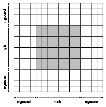
The number of guard cells needed depends upon the interpolation scheme and differencing stencil used for the hydrodynamics algorithm; for the explicit PPM algorithm distributed with FLASH, four guard cells are needed in each direction, as illustrated in Figure 6.

Figure 6: A simple computational domain showing varying levels of refinement. The dotted lines around one block outline the guardcells for that block.

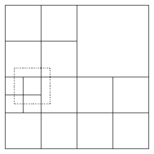
PARAMESH handles the filling of guard cells with information from other blocks or a user-specified external boundary routine. If a block's neighbor has the same level of refinement, PARAMESH fills its guard cells using a direct copy from the neighbor's interior cells. If the neighbor has a different level of refinement, the neighbor's interior cells are used to interpolate guard cell values for the block. If the block and its neighbor are stored in the memory of different processors, PARAMESH handles the appropriate parallel communication (blocks are not split between processors). PARAMESH supports only linear interpolation for guard cell filling at jumps at refinement, but it is easily extended to allow other interpolation schemes. In FLASH, several different interpolation methods can be chosen at setup time. Each interpolation scheme is stored in a subdirectory under /source/mesh/paramesh_nobarr. Once each block's guard cells are filled, it can be updated independently of the other blocks. PARAMESH also enforces flux conservation at jumps in refinement, as described by Berger and Colella (1989). At jumps in refinement, the fluxes of mass, momemtum, energy (total and internal), and species density in the fine cells across boundary cell faces are summed and passed to their parent. The parent and the neighboring cell are at the same level of refinement (because PARAMESH limits the jumps in refinement to be one level between blocks). The flux in the parent that was computed by the more accurate fine zones is taken as the correct flux through the interface, and it is passed to the corresponding coarse face on the neighboring block (see Figure 7). The summing allows a geometrical weighting to be implemented for non-Cartesian geometries, which ensures that the proper corrected flux is computed.

Figure 7: Flux conservation at a jump in refinement. The fluxes in the fine cells are added and replace the coarse cell flux (F)

Each processor decides when to refine or derefine its blocks by computing a user-defined error estimator for each block. Refinement involves creation of either zero or 2^d refined child blocks, while derefinement involves deletion of a block and all its siblings (2^d blocks). As child blocks are created, they are temporarily placed at the end of the processor's block list. After the refinements and derefinements are complete, the blocks are redistributed among the processors using a work-weighted Morton space-filling curve in a manner similar to that described by Warren and Salmon (1987) for a parallel treecode. An example Morton curve is shown in Figure 8.

Figure 8: Morton space-filling curve

During the distribution step each block is assigned a work value (an estimate of the relative amount of time required to update the block). The Morton number of the block is then computed by interleaving the bits of its integer coordinates as described by Warren and Salmon (1987); this determines its location along the space-filling curve. Finally, the list of all blocks is partitioned among the processors using the block weights, equalizing the estimated workload of each processor.

6.2.1  Dividing the computational domain

Dividing the domain is the first step in the mesh-generation process. This routine is responsible for creating the initial top-level block(s) and setting the neighbors of these blocks correctly. These initial blocks then form the top of the tree, and new blocks may be created by refining these top blocks.

By default, FLASH generates an initial mesh with only one top-level block. There are times when this is inconvenient; for instance, when simulating a domain longer in one dimension than the other while wanting equal spatial resolution in each dimension.

divide_domain() creates an initial mesh of nblockx * nblocky * nblockz top level blocks, where nblockx, nblocky, and nblockz are runtime parameters which default to 1. These blocks are all created on one processor, and thus the total number of these top-level blocks may not exceed the compiled-in parameter MAXBLOCKS.

Since divide_domain() is responsible for setting the neighbors of top-level blocks correctly (to either other top-level blocks or to external boundary conditions calcluated by tot_bnd), this is also where the periodic boundary conditions are initially set up. If periodic boundary conditions are set in (for instance) the x-direction, the blocks that are first in the x-direction are set to have as their left-most neigbor the blocks that are last in the x-direction, and vice versa. Thus, when the guard cell filling is performed, the periodic boundary conditions are automatically maintained.

6.2.2  Message buffering

In the maintenance of the tree structure during refinement or derefinement, many small messages must be sent between processors. On any system with a non-negligable latency time for sending messages, communications costs can be significantly reduced by batching these many small messages into fewer large messages.

The routines in batchsend.F90 and batchsend_dbl.F90 do simple message buffering. In several amr routines, all blocks need to send to their neighbors a small number of pieces of data along with a tag, as well as recieve some data. The processors they are to send to and recieve from are known ahead of time. The routines b_int_sendrecv(), b_logical_sendrecv(), and b_dbl_sendrecv() take as input arrays containing the messages, tags, and processors to send or recieve from, and batch them so that as few messages as possible go between processors.

Because of the amount of copying and memory allocation involved in the process, this buffering does have a cost, and thus under some circumstances may produce a performance loss rather than gain. Thus, the message buffering may be turned on or off with the logical runtime parameter msgbuffer, which is .false. by default.

6.3  Using cylindrical coordinates

By default, FLASH uses a Cartesian geometry when discretizing the computational domain. The only other geometry currently available in FLASH is 2-d cylindrical (r,z) coordinates. This coordinate system is useful for problems that are axisymmetric. In FLASH, it is assumed that the cylindrical radial coordinate is in the `x'-direction, and the cylindrical z-coordinate is in the `y'-direction. To run FLASH with cylindrical coordinates, the igeomX runtime parameters must be set properly:

    igeomx = 1
    igeomy = 0
    igeomz = 3

These parameters are interpreted by the hydrodynamics solvers and add the necessary geometrical factors to the divergence terms.

As discussed in the AMR section, to ensure conservation at a jump in refinement, a flux correction step is taken. Here we use the fluxes leaving the fine zones adjacent to a coarse zone to make a more accurate flux entering the coarse zone.

Figure 9 shows a jump in refinement along the cylindrical `z' direction. When performing the flux correction step at a jump in refinement, we must take into account the area of the annulus that each flux passes through to do the proper weighting. We define the cross-sectional area the z-flux passes through as

A = p(rr2 - rl2),

(12)

where r_r and r_l are the zone maxima and minima in the radial direction respectively. The flux entering the coarse zone above the jump in refinement is corrected to agree with the fluxes leaving the fine zones that border it. This correction is weighted according to the areas:

f3 =  A1 f1 + A2 f2 A3

(13)

Figure 9: Cartoon showing two fine zones and a coarse zone at a jump in refinement in the cylindrical `z' direction. The block boundary has been cut apart here for illustrative purposes. The fluxes out of the fine blocks are shown as f1 and f2. These will be used to compute a more accurate flux entering the coarse flux f3. The area that the flux passes through in shown as the annulus at the top of each fine zone, and below the coarse zone.

For fluxes in the radial direction, the cross-sectional area is independent of the height, z, so the corrected flux is simply taken as the average of the flux densities in the adjacent finer zones.

6.4  Using a uniform grid

By default, FLASH will run a problem on an adaptive mesh, keeping the level of refinement of a block between lrefine_min and lrefine_max. Sometimes it is useful to run a problem with a uniform mesh. While there is no explicitly uniform mesh module distributed with FLASH, the paramesh module can be run in a uniform `mode', which will have only slightly more overhead that a purely uniform mesh module. The basic steps to set this up are outlined below.

A typical problem in FLASH is set up with a single block at the top of the tree. As the refinement criteria is applied to the initial conditions, this block and any children are refined to create the initial mesh. If you are running on a uniform grid, there is no need to carry around the entire tree hierachry, only the leaf blocks are needed. To get around this, we can use the divide_domain functionality (see section ??) to create enough as many top level blocks as are needed to satisfy our resolution needs. This is accomplished by using the nblockx, nblocky, and nblockz runtime parameters to specify how many blocks to create in each direction.

Since you are placing the same resolution everywhere in the domain, it is no longer advantageous to use small blocks. Instead, the number of zones in a block can be increased, which will reduce the memory overhead (ratio of guardcells to interior zones in a single block). At present, the only way to do this in FLASH is to modify physicaldata.fh, and increase the values of nxb, nyb, and nzb. Please note, some sections of the code assume that these quantities are even.

The number of computation zones in each direction can be computed as:

Nxzones = nblockx ×nxb

(14)

for the x-direction. Adjust nxb and nblockx to get the desired number of zones in the x-direction (and similarily for the other coordinate directions). You can then set lrefine_max = lrefine_min = 1.

Since there will be no refinement in the problem, the next step is to instruct the code to no longer check for refinement. This is accomplished by setting nref to a very large number. nref is the frequency (in time steps) to check the refinement criteria, and defaults to 2.

Finally, since there will be no jumps in refinement, the flux conserveration step is not necessary. This can be eliminated by commenting out the FLUX preprocessor definition in hydro_sweep. This will instruct the code to skip over the conservation step.

7  Hydrodynamics modules

The hydro module solves Euler's equations for compressible gas dynamics in one, two, or three spatial dimensions. These equations can be written in conservative form as

¶r ¶t + Ñ ·( rv ) = 0 (15)  ¶rv ¶t + Ñ ·( rv v ) + Ñ P = rg (16)  ¶rE ¶t + Ñ ·[ ( rE + P ) v ] = rv ·g , (17)

where r is the fluid density, v is the fluid velocity, P is the pressure, E is the sum of the internal energy e and kinetic energy per unit mass,

E = e+  1 2 |v|2 ,

(18)

g is the acceleration due to gravity, and t is the time coordinate. The pressure is obtained from the energy and density using the equation of state. For the case of an ideal gas equation of state, the pressure is given by

P = (g- 1) re ,

(19)

where g is the ratio of specific heats. More general equations of state are discussed in Section 9.2.1.

In regions where the kinetic energy greatly dominates the total energy, computing the internal energy using

e = E -  1 2 |v|2

(20)

can lead to unphysical values, primarily due to truncation error. This results in inaccurate pressures and temperatures. To avoid this problem, we can separately evolve the internal energy according to

¶re ¶t + Ñ·[ (re+ P )v ] - v·ÑP = 0 .

(21)

If the internal energy is a small fraction of the kinetic energy (determined via the runtime parameter eint_switch), then the total energy is recomputed using the internal energy from equation (21) and the velocities from the momentum equation. Numerical experiments using the PPM solver included with FLASH showed that using equation (21) when the internal energy falls below 10^-4 of the kinetic energy helps avoid the truncation errors, while not affecting the dynamics of the simulation.

For reactive flows, a separate advection equation must be solved for each chemical or nuclear species:

¶rXl ¶t + Ñ ·( rXl v ) = 0 ,

(22)

where X_l is the mass fraction of the lth species, with the constraint that å_l X_l = 1. FLASH will enforce this constraint if you set the runtime parameter irenorm equal to 1. Otherwise, FLASH will only restrict the abundances to fall between smallx and 1. The quantity rX_l represents the partial density of the lth fluid. The code does not explicitly track interfaces between the fluids, so a small amount of numerical mixing can be expected during the course of a calculation.

All hydrodynamic modules, as well as the MHD module described in Section 8, supply the runtime parameters and solution variables described in Tables 6 and 7. Two hydrodynamic modules are included. The first, discussed in Section 7.1, is based on the directionally split Piecewise-Parabolic Method (PPM) and makes use of second-order Strang time splitting. The second, discussed in 7.2, is based on Kurganov methods and can make use of Strang splitting or Runge-Kutta time advancement. Explicit, directionally split solvers like the PPM solver make use of the additional runtime parameter described in Table 8.

Table 11: Runtime parameters used with the hydrodynamics (hydro) modules.

Variable	Type	Default	Description
eint_switch	real	10-4	If e < eint_switch ·1/2|v|2, use the internal energy equation to update the pressure
irenorm	integer	0	If equal to one, renormalize multifluid abundances following a hydro update; else restrict their values to lie between smallx and 1.

Table 12: Solution variables used with the hydrodynamics (hydro) modules.

Variable	Attributes	Description
dens	ADVECT NORENORM CONSERVE	density
velx	ADVECT NORENORM NOCONSERVE	x-component of velocity
vely	ADVECT NORENORM NOCONSERVE	y-component of velocity
velz	ADVECT NORENORM NOCONSERVE	z-component of velocity
pres	ADVECT NORENORM NOCONSERVE	pressure
ener	ADVECT NORENORM NOCONSERVE	specific total energy (T+U)
temp	ADVECT NORENORM NOCONSERVE	temperature

Table 13: Runtime parameters used with the explicit hydrodynamics (hydro/explicit) modules.

Variable	Type	Default	Description
cfl	real	0.8	Courant-Friedrichs-Lewy (CFL) factor; must be < 1 for stability in explicit schemes

7.1  The Piecewise-Parabolic Method (PPM)

7.1.1  Algorithm

FLASH includes a directionally split Piecewise-Parabolic Method (PPM) solver descended from the PROMETHEUS code (Fryxell, Müller, and Arnett 1989). PPM is described in detail in Woodward and Colella (1984) and Colella and Woodward (1984). It is a higher-order version of the method developed by Godunov (1959). Godunov's method uses a finite-volume spatial discretization of the Euler equations together with an explicit forward time difference. Time-advanced fluxes at cell boundaries are computed using the analytic solution to Riemann's shock tube problem at each boundary. Initial conditions for each Riemann problem are determined by assuming the nonadvanced solution to be piecewise constant in each cell. Using the Riemann solution has the effect of introducing explicit nonlinearity into the difference equations and permits the calculation of sharp shock fronts and contact discontinuities without introducing significant nonphysical oscillations into the flow. Since the value of each variable in each cell is assumed to be constant, Godunov's method is limited to first-order accuracy in both space and time.

PPM improves on Godunov's method by representing the flow variables with piecewise parabolic functions. It also uses a monotonicity constraint rather than artificial viscosity to control oscillations near discontinuities, a feature shared with the MUSCL scheme of van Leer (1979). Although this could lead to a method which is accurate to third order, PPM is formally accurate only to second order in both space and time, as a fully third-order scheme proved not to be cost-effective. Nevertheless, PPM is considerably more accurate and efficient than most formally second-order algorithms.

PPM is particularly well-suited to flows involving discontinuities, such as shocks and contact discontinuities. The method also performs extremely well for smooth flows, although other schemes which do not perform the extra work necessary for the treatment of discontinuities might be more efficient in these cases. The high resolution and accuracy of PPM are obtained by the explicit nonlinearity of the scheme and through the use of intelligent dissipation algorithms, such as monotonicity enforcement, contact steepening, and interpolant flattening. These algorithms are described in detail by Colella and Woodward (1984).

A complete description of PPM is beyond the scope of this user's guide. However, for comparison with other codes, we note that the implementation of PPM in FLASH 2.x uses the direct Eulerian formulation of PPM and the technique for allowing nonideal equations of state described by Colella and Glaz (1985). For multidimensional problems, FLASH 2.x uses second-order operator splitting (Strang 1968).

7.1.2  Usage

The hydro/explicit/split/ppm module supplies the runtime parameters described in Table 9.

Table 14: Runtime parameters used with the PPM (hydro/explicit/split/ppm) module.

Variable	Type	Default	Description
epsiln	real	0.33	PPM shock detection parameter e
omg1	real	0.75	PPM dissipation parameter w1
omg2	real	10	PPM dissipation parameter w2
igodu	integer	0	If set to 1, use the Godunov method (completely flatten all interpolants)
vgrid	real	0	Scale factor for dissipative grid velocity
nriem	integer	10	Max number of iterations to use in Riemann solver
rieman_tol	real	10-5	Convergence factor for Riemann solver
cvisc	real	0.1	Artificial viscosity constant
oldvisc	boolean	.true.	If .true., use the original PROMETHEUS artificial viscosity; else use a newer one developed by Müller and Plewa

7.1.3  Diffusion

Any of several diffusive processes can be added to the Euler equations in the PPM module. All of these are treated explicitly in FLASH, and follow the same approach: a diffusive flux is calculated by assuming that the diffusive flux of a quantity is proportional to the gradient of the quantity. The gradient is calculated by finite difference. The fluxes are then calculated and added to the fluxes generated by the PPM module. This addition is done before any of the zones are updated in the hydro step. This ensures conservation, since the total flux (including the diffusive flux) will be corrected during the flux conservation step.

To include a diffusive process, you must modify your Modules file to use
source/hydro/explicit/split/ppm/diffuse. Then the logical runtime parameters
diffuse_therm, diffuse_visc, and diffuse_species should be set to .TRUE. or .FALSE. depending on whether you wish to include these diffusive terms or not in your simulation.

7.1.3.1  Thermal Diffusion  

The energy equation in the PPM module can be modified to include thermal diffusion:

¶rE ¶t + Ñ ·(rE + P ) v = rv ·g + Ñ ·(s(Xi, r, T) Ñ T) + enuc(Xi,r, T),

(23)

where s(X_i, r, T) is the conductivity and

Fheat = - s(Xi, r, T) Ñ T

(24)

is the explicit heat flux.

There are several conductivity modules available for use with this routine in
source/materials/conductivity, and one of these must be included in your Modules file. conductivity/stellar uses a conductivity appropriate for the degenerate matter of stellar interiors. In conductivity/constant the heat conductivity is assumed constant - s is set equal to the runtime parameter conductivity_constant. In conductivity/constant-diff, the thermal diffusivity (l = [(s)/(rc_p)]) is kept equal to the runtime parameter diff_constant. This is equivalent to diffusing temperature directly, e.g.

¶T ¶t + Ñ·T v = Ñ·( lÑT )

(25)

7.1.3.2  Viscosity  

With viscosity, it is velocity which is diffused:

rv rt + Ñ ·r v v + Ñ P = rg + Ñ ·(nÑv)

(26)

The fluxes are calculated as in the thermal diffusion, although there is one flux for each velocity component. The viscosity, n, is assumed constant and set by the runtime parameter diff_visc_nu. Total energy fluxes are not updated by viscosity, as it assumed the effect is small.

7.1.3.3  Species Diffusion  

The species diffusion diffuses number density of species. Thus, there are ionmax fluxes updated, and they are controlled by an assumed constant diffusivity diff_spec_D.

¶rXi ¶t + Ñ ·(rXi v) = Ñ ·(D Ñ rXi)

(27)

7.2  The Kurganov hydrodynamics module

The two Kurganov schemes are implemented in the kurganov hydro module, which is compatible with all the new driver modules. The module is organized as follows. The subroutine hydro_3d is essentially a wrapper to the subroutines kurganov_block_x, kurganov_block_y, and kurganov_block_z. These three subroutines implement the reconstruction step for each of the spatial dimensions, and call kurganov_line, which calculates either the KT or KNP numerical fluxes.

7.2.1  Algorithm

The new hydro module provides two of Kurganov's high-resolution central schemes, each second-order accurate. These spatial discretization methods for the advective terms provide robust shock-capturing without characteristic decompositions, which makes them relatively inexpensive compared to other shock-capturing schemes. However, they may have a lower critical time step for stability and higher dissipation as a result.

Kurganov and his collaborators have developed a a class of numerical methods for hyperbolic conservation laws. Compared to other methods for such systems, the Kurganov methods are simple and inexpensive because they do not rely on characteristic decompositions or Riemann solvers; the only information they require from the equations is the maximum and minimum signal propagation speeds. The Kurganov methods evolved from methods developed by Tadmor and his colleagues, but differ in that staggered grids are not used in the implementation, only as a device in the derivation of the schemes.

There are two parts to each Kurganov method, (i) reconstruction of the conserved variables, which provides cell interface values, and (ii) computation of the interface flux from those interface values. Various second- and third-order reconstruction algorithms have been developed; one-dimensional reconstructions can be extended dimension-by-dimension, but some multidimensional third-order reconstructions have been proposed. Two formulas are available for computing the fluxes from the interface values. For the first numerical flux, several wave speeds were represented by a single estimate, the maximum magnitude of the eigenvalues of the flux Jacobian (Kurganov and Tadmor 2000). Later two estimates (maximum and minimum eigenvalues) were used, resulting in an improved numerical flux with reduced numerical dissipation (Kurganov, Noelle, and Petrova 2001).

Next the second-order reconstruction used in the new hydro module will be described. The reconstruction is one-dimensional, and is presented for an equispaced mesh. An arbitrary mesh cell is referred to by subscript i. The reconstruction uses the cell-averaged conserved variables, U_i, at nearby cells to produce values of the conserved variables at the left and right sides of each cell interface, U^l_i+[ 1/2] and U^r_i+[ 1/2], respectively. To update a given cell fluxes at two interfaces must be computed, so for the reconstruction presented, the this update requires a five-point stencil.

The first step is to compute limited slopes, (U_x)_i:

(Ux)i = minmod é ë q( Ui+1 - Ui ), q( Ui - Ui-1 ),  1 2 ( Ui+1 - Ui-1 ) ù û

(28)

where the minmod function returns the smallest argument in magnitude if all arguments are the same sign, and zero if they are not. The parameter 1 £ q £ 2 gives some control over the limiter. The minmod limiter is recovered for q = 1, and is one of the most diffusive limiters. The monotonized central limiter (Colella and Woodward 1984) is specified for q = 2; it is significantly less dissipative, and recommended for most cases. Other limiters may also be used to compute the slopes; each has its pros and cons.

Once the slopes have been determined, the interface values are calculated by

Uli+[ 1/2] = Ui +  1 2 (Ux)i (29) Uri+[ 1/2] = Ui+1 -  1 2 (Ux)i+1. (30)

Then, on each side of the interface, the speed of sound is computed. This requires the density, mass fractions, and internal energy to be computed; then the equation of state module is called, which returns the pressure and the ratio of specific heats. Finally, the speeds of sound c^l_i+[ 1/2] and c^r_i+[ 1/2] are computed by c = (gP/r)^[ 1/2].

The Kurganov-Noelle-Petrova (KNP) numerical flux is defined by

Fi+[ 1/2] =   a-i+[ 1/2] F(Uri+[ 1/2]) + a+i+[ 1/2] F(Uli+[ 1/2]) a+i+[ 1/2] + a-i+[ 1/2] + ai+[ 1/2] ( Uri+[ 1/2] - Uli+[ 1/2] )

(31)

where, for the x-direction,

a+i+[ 1/2] = max ( 0, uli+[ 1/2] + cli+[ 1/2], uri+[ 1/2] + cri+[ 1/2] ) (32) a-i+[ 1/2] = - min ( 0, uli+[ 1/2] - cli+[ 1/2], uri+[ 1/2] - cri+[ 1/2] ) (33) ai+[ 1/2] = - ( a+i+[ 1/2] a-i+[ 1/2] ) / ( a+i+[ 1/2] + a-i+[ 1/2] ). (34)

Equations (32) and (33) are specific to the x-direction because u, the x-component of the velocity, appears; for the y- and z-directions, the appropriate velocity components, v and w, respectively should replace u.

The Kurganov-Tadmor (KT) numerical flux is

Fi+[ 1/2] =  1 2 [ F(Uri+[ 1/2]) + F(Uli+[ 1/2]) + ai+[ 1/2] ( Uri+[ 1/2] - Uli+[ 1/2] ) ]

(35)

where, for the x-direction,

ai+[ 1/2] = max ( |uli+[ 1/2] + cli+[ 1/2]|, |uri+[ 1/2] + cri+[ 1/2]| ).

(36)

As in eqns. (32) and (33), the appropriate velocity components should be used in eq. (36) for the y- and z-directions.

7.2.2  Usage

The hydro_3d subroutine was written as generally as possible - with minimal modification, it can be used as a wrapper for most shock-capturing schemes which compute numerical fluxes. It accepts, as an argument, the spatial direction - x, y, z, or all - for which the fluxes should be computed. It can therefore be used with time advancement methods based on directional splitting. In order, the tasks handled by hydro_3d include:

1. fill guard cells
2. loop over blocks:

   1. eos call for guard cells
   2. get field data
   3. get mesh data
   4. for each applicable direction:

      1. get fluxes on equispaced grid: call kurganov_block for the appropriate direction
      2. apply geometry factors
      3. update global DU or locally update solution, depending on formulation
      4. save block boundary fluxes for AMR conservation
3. AMR flux conservation
4. loop over blocks:

   1. apply corrections from AMR flux conservation

By managing all these tasks, all the interaction between the Kurganov shock-capturing schemes and the rest of the FLASH code framework is encompassed in hydro_3d.

The kurganov module accepts two runtime parameters, listed in table 10. The integer knp selects which numerical flux formula is to be used, KNP or KT. The real-valued lim_theta is q in eq. (28); lower values result in more damping, higher values in less, within the range listed in the table. The runtime parameter cfl is common to all hydro modules; table 10 lists only those specific to the Kurganov schemes. Because of the reconstruction, a five-point stencil is required at each mesh cell; consequently, two guard cells are required for a block. Corner guard cells are not required since the reconstruction is one-dimensional.

Table 15: Runtime parameters used with the kurganov hydro module.

Para. name	Type	Default	Description
knp	integer	1	Specifies KNP numerical flux is to be used; for KT, set knp=0
lim_theta	real	2.0	Adjusts slope limiter; 1.0 £ lim_theta £ 2.0; choose 1.0 for minmod limiter, 2.0 for monotonized centered limiter

7.2.2.1  Interaction with delta and state-vector driver modules  

New driver, formulation, and hydro modules have been implemented in a manner which maximizes flexibility. In this section the interaction between these three module classes is explained. More generally, though, the new hydro module represents all physics modules; it is an example of how other modules can be written so they can be used with the new driver and formulation modules. To use the new methods, the user should specify their inclusion through the Modules file, as described below.

The new hydro module, kurganov, can be used with drivers written in either delta or state-vector formulations. All physics modules can be written with this feature, and the kurganov module can be used as a guide for doing so.

On each block, the hydro module does the following. The contribution of the module, L_hydro(U), is computed. If a delta formulation time advancement has been specified, then L_hydro(U) is added to the global DU. If a state-vector formulation time advancement is being used, calls to update the solution on the block from L_hydro(U) are made. In both cases, the formulation module provides the subroutines for these actions. The line for the Modules file to specify the Kurganov scheme is:

/hydro/explicit/delta_form/kurganov

The directory names for some of the new modules are misleading. All the new time advancements are in a directory named delta_form, regardless of their formulation; this directory will be renamed multi_form in the near future. Similarly, /hydro/explicit/delta_form will be renamed /hydro/explicit/multi_form.

7.2.2.2  Caveats  

At present, the compatibility of the new modules with the rest of the FLASH code is limited. The new modules are incompatible with the default hydro module, which actually implements parts of the Strang splitting time advancement in addition to the PPM spatial discretization. The time advancements implemented in the delta formulation are not compatible with physics modules which update the variables, and those implemented in the state-vector formulation have not been tested with the other physics modules; these deficiencies are being addressed. Currently only Cartesian coordinates are supported by the new hydro module. The new modules have been extensively tested only for a nonreacting, single component gas (ionmax=1) using the gamma-law equation of state.

8  The magnetohydrodynamics module

The magnetohydrodynamics module included with the FLASH code solves the equations of ideal MHD. As discussed in 8.1, the MHD module replaces the hydrodynamics module in simulations of magnetized fluids. The two modules are conceptually very similar, and they share the same algorithmic structure. In the current version of the FLASH code, the MHD module is a submodule of the hydrodynamics module. This hierarchy will change in future releases of the code, and hydro and MHD modules will be placed at the same level in the source module tree.

The currently released version of the MHD module uses directional splitting to evolve the equations of ideal magnetohydrodynamics. As the hydro module does, the MHD module (mhd.F90, mhd_3d.F90) makes three sweeps (functions mhd_x(), mhd_y() and mhd_z()) to advance physical variables from one time level to another one. In each sweep, the module uses AMR functionality to fill in guard cells and impose boundary conditions. Then it reconstructs characteristic variables (mhd_interpolate()) and uses these variables to compute time-averaged interface fluxes of conserved quantities. In order to enforce conservation at jumps in refinement the module calls amr_flux_conserve(), which redistributes affected fluxes using appropriate geometric area factors. Finally, the module updates the solution and calls eos3d() to ensure that the solution is thermodynamically consistent.

After all sweeps are completed the MHD module enforces magnetic field divergence cleaning. Two options are available: diffusive and elliptic projection cleaning. In order to select a particular method, the user must respectively specify either mhd/divb_diffuse or mhd/divb_project in his or her problem Config file. The default method is diffusive.

The interface of the MHD module is minimal. The module honors most of the hydro module interface functions and shares several common parameters. The most significant of them is the cfl number. At the time of this writing the module introduces only two MHD-specific runtime parameters:

killdivb - a logical variable that specifies whether divergence cleaning should be enabled or disabled. The default value is TRUE.
divbcleanfactor - a real variable between 0 and 1 that specifies the strength of divergence cleaning; 0 corresponds to no cleaning and 1 corresponds to maximum cleaning. The default value is 1.

All other MHD-specific parameters are encapsulated in the MHD module in mhd.F90.

8.1  Algorithm

The magnetohydrodynamic (MHD) module in the FLASH 2.0 code is based on a finite-volume, cell-centered method that was recently proposed by Powell et al. (1999). This particular choice for the solver is made so that the solver complies with the data structure layout required by the existing hydrodynamics module. As a result of this choice, the MHD module in the FLASH 2.0 code is fully compatible and is, in fact, swappable with the hydro module.

The MHD module in the FLASH 2.0 code solves the equations of compressible magnetohydrodynamics in one, two and three dimensions. Written in non-dimensional (hence without 4p or m₀ coefficients), conservation form these equations are

¶r ¶t + Ñ·(rv) = 0 (37)  ¶rv ¶t + Ñ·(rvv-BB)+Ñ(p+B2/2) = rg (38)  ¶rE ¶t + Ñ·(v(rE+p+B2/2)-B(v·B)) = rg·v (39)  ¶B ¶t + Ñ·(vB-Bv) = 0, (40)

where

E =  1 2 v2+e+  1 2  B2 r

(41)

is the specific total energy, r is the density of a magnetized fluid, v is the fluid velocity, p is the fluid thermal pressure, e is the specific internal energy, B is the magnetic field and g is the body force per unit mass, for example due to gravity. The thermal pressure is a scalar quantity, so that the code is suitable for simulations of ideal plasmas in which magnetic fields are not too strong so as to caus e temperature anisotropies. As in regular hydrodynamics, the pressure is obtained from the internal energy and density using the equation of state. In the present version, the MHD module supports only an ideal equation of state

p = (g-1)re,

(42)

where g is the adiabatic index. This restriction will be removed in subsequent releases of the code, and the MHD module will support general equations of states as well as multi-species fluids.

The above equations of ideal magnetohydrodynamics are solved using a high-resolution, finite-volume numerical scheme with MUSCL-type (van Leer 1979) limited gradient reconstruction. In order to maximize the accuracy of the solver the reconstruction procedure is applied to characteristic variables. Since this may cause certain variables such as density and pressure to fall out of physically meaningful bounds, extra care is taken in the limiting step to prevent this from happening. All other variables are calculated in the module from the interpolated characteristic variables.

In order to resolve discontinuous Riemann problems that occur at computational cell interfaces, the code employs a Roe-type solver derived in Powell et al. (1999). This solver provides full characteristic decomposition of the ideal MHD equations, and is therefore particularly useful for plasma flow simulations that feature complex wave interaction patterns. The time integration in the MHD module is done using a second-order, one-step method due to Hancock (Toro 1997). For linear systems with unlimited gradient reconstruction this method can be shown to coincide with the classic Lax-Wendroff scheme.

A difficulty particularly associated with solving the MHD equations numerically lies in the solenoidality of the magnetic field. The notorious Ñ·B =0 condition, a strict physical law, is very hard to satisfy in discrete computations. Being only an initial condition of the MHD equations it enter s the equations indirectly and is not therefore guaranteed to be generally satisfied unless special algorithmic provisions are made. Without discussing this issue in much detail, which goes well beyond the scope of this user's guide (for example, see Tóth (2000) and references therein), we will remind that there are three commonly accepted methods to enforce the Ñ·B condition: the elliptic projection method (Brackbill and Barnes 1980), the constrained transport method (Evans and Hawley 1988) and the truncation-level error method (Powell et al. 1999). In the FLASH 2.0 code, the truncation-error and elliptic cleaning methods are implemented.

In the truncation-error method, the solenoidality of the magnetic field is enforced by including several terms proportional to Ñ·B. This removes the effects of unphysical magnetic tension forces parallel to the field and stimulates passive advection of magnetic monopoles if these are spuriously created. In many applica tions, this method has been shown to be efficient and sufficient way to generate solutions of high physical quality. However, it has also been shown (Tóth, 2000) that this method can sometimes, for example in strongly discontinuous and stagnated flows, lead to accumulation of magnetic monopoles whose strength is sufficient to corrupt the physical quality of computed solutions. In order to eliminate this deficiency, the FLASH 2.0 code also uses a simple yet very effective method originally due to Marder (1987) to destroy the magnetic monopoles on the scale on which they are generated. In this method, a diffusive operator proportional to ÑÑ·B is added to the induction equation, so that the equation becomes

¶B ¶t +Ñ·(vB-Bv) = -vÑ·B+hÑÑ·B,

(43)

with the artificial diffusion coefficient h chosen to match that of grid numerical diffusion. In the FLASH code, h = [(l)/2]([ 1/(Dx)]+[ 1/(Dy)]+[ 1/(Dz)])^-1, where l is the largest characteristic speed in the flow. Since the grid magnetic diffusion Reynolds number is always on the order of unity, this operator locally destroys magnetic monopoles at the rate at which they are created. Recent numerical experiments (Linde and Malagoli, submitted; Powell et al. (2001)) indicate that this approach can very effectively bring the strength of spurious magnetic monopoles to acceptably low levels, so that generated solutions are guaranteed to remain physically consistent. The entire Ñ·B control process is local and very inexpensive compared to other methods. Moreover, one can show that this process is asymptotically convergent (Munz et al., 2000), and each of its applications is equivalent to one Jacobi iteration in solving the Poisson equation in the elliptic projection method. The caveat is that this method only suppresses but does not completely eliminate magnetic monopoles. Whether this is acceptable depends on a particular physical problem.

In order to eliminate magnetic monopoles completely, the FLASH 2.0 code includes an elliptic projection method. In this method, the unphysical divergence of magnetic field can be removed to any desired level down to machine precision. This is achieved by solving a Poisson equation for a correcting scalar field whose gradient removes contaminated field components when subtracted from the magnetic field. The Poisson solver needed for this operation is the multigrid solver that is also used by the gravity module.

9  Material properties modules

FLASH has the ability to track multiple fluids, each of which can have their own properties. The materials module handles these, as well as other things like EOS, composition, and conductivities.

9.1  The multifluid database

To access any of the fluid properties, you must use the multifluid database. This can be accomplished in any FLASH routine by including the line:

use multifluid_database

along with any of the other modules you have included. This module provides interface functions that can be used to set or query a fluid's properties. As with the other databases in FLASH, most of the properties have both a string name and an integer key that can be used in the database call. Calling the function with the integer key will be faster, since it avoids expensive string comparisons. The available properties are listed in table 11.

Table 16: Properties available through the multifluid database.
name	integer key	property	data type
``name"	N/A	fluid name	string
``short name"	N/A	chemical symbol	string
``num total"	mf_prop_A	A	real
``num positive"	mf_prop_Z	Z	real
``num neutral"	mf_prop_N	N	real
``num negative"	mf_prop_E	E	real
``binding energy"	mf_prop_Eb	binding energy	real
``adiabatic index"	mf_prop_gamma	gamma	real

Once the multifluid database is initialized (usually by the materials/composition module function init_materials(), the integer nfluids is publicly available, giving the number of fluids carried by FLASH.

An example of using the multifluid database to define two fluids two be tracked by FLASH is provided by the example setup, discussed in 2.2.

We now briefly discuss the various interfaces to the multifluid database. Many of these functions are overloaded to accept either string or integer properties (as listed in the table above), or to include optional arguments. We only discuss the generic interface here.

• add_fluid_to_db(name, short_name, properties, status)

  A quick way to set a number of properties for an individual fluid in a single subroutine call. Looks for the next uninitialized fluid ( init_mfluid_db() sets the names of all fluids to UNINITIALIZED) and sets its properties according to the values specified in the subroutine call. Properties can be specified in the order A, Z, N, E, ... or by keyword. For example,

  call add_fluid_to_db ("helium", "He", A=4., Z=2., N=2.)
  
  

  Properties not specifically initialized are set to 0. The status parameter is an optional status variable.

  This function call is usually used when initializing the fluids in FLASH. Each composition sets the properties for all the fluids in the routine init_materials().

• set_fluid_property(f, p, v, status)

  Set the property p of fluid f to value v. The fluid, f can be specified either using its string name or index. p is either a string identifier or integer key specifying the property.. The value v can be real-valued or string-valued, depending on the property being modified. status is an optional variable which will be set to 0 if the operation was successful, -1 if not. Reasons why the operation can fail include: f out of bounds if f is an index; f not found if f is a string name; p is not a valid property identifier; v is not a valid value for the given property.

• get_fluid_property(f, p, v, status)

  Like the setting version, but v now receives the value instead of setting it.

• get_mfluid_property(p, v, status)

  Return the value of the property p for all defined fluids. v must be an array of the correct type. status is an optional exit status variable. v is filled with values up to the minimum of (its size, number of fluids).

• find_fluid_index(f, i)

  Find the database index i of a fluid named f. If init_mfluid_db() has not been called, or if the fluid name is not found, this function terminates with an error. Errors are signaled by setting i to MFLUID_STATUS_FAIL.

• query_mfluid_sum(p, w, v, status)

  Given a property name p and an array of weights w, return the weighted sum of the chosen property in v. w should be an array of length equal to the number of fluids in the database, or else a one-element array. Typically, the weights used are the mass fractions of each of the fluids in the database. If it is neither, or if the named property is invalid, the routine terminates. The optional status variable is set to MFLUID_STATUS_OK or MFLUID_STATUS_FAIL depending on whether the summing operation was successful.

• query_mfluid_suminv(p, w, v, status)

  Same as query_mfluid_sum(), but compute the weighted sum of the inverse of the chosen property.

  For example, the average atomic mass of a collection of fluids is typically defined as:
  

  1 - A = å  Xi Ai

  (44)

  where X_i is the mass fraction of species i, and A_i is the atomic mass of that species. To compute [`A] using the multifluid database, one would use the following lines:

        call query_mfluid_suminv(mf_prop_A, xn(:), abarinv, error)
        abar = 1.e0 / abarinv
  
  

  where xn(:) is an array of the mass fractions for each species in FLASH.
• query_mfluid_sumfrc(p, w, v, status)

  Same as query_mfluid_sum(), but compute the weighted sum of the chosen property divided by the total number of particles (A).

• query_mfluid_sumsqr(p, w, v, status)

  Same as query_mfluid_sum(), but compute the weighted sum of the square of the chosen property.

• init_mfluid_db()

  Initialize the multifluid database. If this has not been called and one of the other routines is called, that routine terminates with an error. The typical FLASH user will never need to call this him-/herself, as this call is part of the init_materials() call in the composition submodule.

• list_mfluid_db(lun)

  List the contents of the multifluid database in a snappy table format. Output goes to the logical I/O unit indicated by the lun parameter.

9.2  Equations of state

The eos module implements the equation of state needed by the hydrodynamical and nuclear burning solvers. Interfaces are provided to operate on an entire block (eos3d), a one-dimensional vector (eos1d), or for a single zone (eos_fcn). Additionally, these functions can be used to find the thermodynamic quantities from either the density, temperature, and composition, or density, internal energy, and composition.

Three sub-modules are available in FLASH 2.0: gamma, which implements a perfect-gas equation of state; multigamma, which implements a perfect-gas equation of state with multiple fluids, each of which can have its own adiabatic index (g), and helmholtz, which uses a fast Helmholtz free-energy table interpolation to handle the same degenerate/relativistic electrons/positrons, and includes radiation pressure and ions (via the perfect gas approximation). Full details of this equation of state are provided in Timmes & Swesty (1999).

9.2.1  Algorithm

As described above, FLASH evolves the Euler equations for compressible, inviscid flow. This system of equations must be closed by an additional equation that provides a relation between the thermodynamic quantities of the gas. This is known as the equation of state for the material, and its structure and properties depend on the composition of the gas.

It is common to call an equation of state (henceforth EOS) routine more than 10⁹ times during the course of a simulation when calculating two- and three-dimensional hydrodynamic models of stellar phenomena. Thus, it is very desirable to have an EOS that is as efficient as possible, yet accurately represents the relevant physics, and considerable work can go into development of a robust and efficient EOS. While FLASH is capable of general equations of state, here we discuss the routines for three equations of state that are supplied with FLASH: an ideal-gas or gamma-law EOS, an EOS for a fluid composed of multiple gamma-law gases, and a tabular Helmholtz free energy EOS appropriate for stellar interiors. The gamma-law EOS consists of simple analytic expressions that make for a very fast EOS routine in both the case of a single gas or a mixture of gases. The Helmholtz EOS includes much more physics and relies on a table look-up scheme for performance. In this section we discuss the physics of these equations of state; the interfaces between the EOS routines and the codes are discussed in 9.2.

FLASH uses the method of Colella & Glaz (1995) to handle general equations of state. General equations of state contain 4 adiabatic indices (Chandrasekhar 1939), but the method of Colella & Glaz parameterizes the EOS and requires only two of the adiabatic indices. The first is necessary to calculate the adiabatic sound speed and is given by

g1 =  P r  ¶P ¶r   .

(45)

The second relates the pressure to the energy and is given by

g4 = 1 +  P re   .

(46)

These two adiabatic indices are stored as the variables gamc and game. All EOS routines must return g₁, and g₄ is calculated from 46.

The gamma-law EOS models a simple ideal gas with a constant adiabatic index g. Here we have dropped the subscript on g because for an ideal gas all adiabatic indices are equal. The relationship between pressure P and density and specific internal energy r and e is

P = (g- 1)re  .

(47)

We also have an expression relating pressure to the temperature T

P =  Na k - A rT

(48)

where N_a is the Avogadro number, k is the Boltzmann constant, and [`A] is the average atomic mass, defined as

1 - A = å i   Xi Ai

(49)

where X_i is the mass fraction of the ith element. Equating these expressions for pressure yields an expression for the specific internal energy as a function of temperature

e =  T Na k - A     .

(50)

Simulations are not restricted to a single ideal gas, however, because the multigamma EOS provides routines for simulations with several species of ideal gases with different gs. In this case, the above expressions hold, but g represents the weighted average adiabatic index calculated from

1 (g- 1) = å i   1 (gi -1)  Xi Ai

(51)

We note that the analytic expressions apply to both the forward (internal energy as a function of density, temperature, and composition) and backward (temperature as a function of density, internal energy and composition) relations. Because the backward relation requires no iteration in order to obtain the temperature, this EOS is quite inexpensive to evaluate. Despite its performance, use of the gamma-law EOS is limited due to its restricted range of applicability for astrophysical flash problems.

The Helmholtz EOS provided with the FLASH distribution contains more physics and is appropriate for addressing astrophysical phenomena in which electrons and positrons may be relativistic and/or degenerate and in which radiation may significantly contribute to the thermodynamic state. This EOS includes contributions from radiation, completely ionized nuclei, and degenerate/relativistic electrons and positrons. The pressure and internal energy are calculated as the sum over the components

Ptot = Prad + Pion + Pele + Ppos + Pcoul

(52)

etot = erad + eion +eele + epos + ecoul   .

(53)

Here the subscripts ``rad,'' ``ion,'' ``ele,'' ``pos,'' and ``coul'' represent the contributions from radiation, nuclei, electrons, positrons, and corrections for Coulomb effects, respectively. The radiation portion assumes a blackbody in local thermodynamic equilibrium, the ion portion (nuclei) is treated as an ideal gas with g  =  5/3, and the electrons and positrons are treated as a non-interacting Fermi gas.

The blackbody pressure and energy are calculated as

Prad =  a T4 3

(54)

erad =   3 Prad r

(55)

where a is related to the Stephan-Boltzmann constant, s_B   =  ac/4, and c is the speed of light. The ion portion of each routine is the ideal gas of equations (47)-(48) with g  =  5/3. The number densities of free electrons N_ele and positrons N_pos in the noninteracting Fermi gas formalism are given by

Nele =  8 pÖ2 h3   me3  c3  b3/2   [ F1/2(h,b)  +  F3/2(h,b) ]

(56)

Npos =  8 pÖ2 h3   me3  c3  b3/2 [ F1/2 ( -h- 2/b, b)  +  b  F3/2 ( -h- 2 /b, b) ] ,

(57)

where h is the Planck constant, m_e is the electron rest mass, b  =  k T / (m_e c²) is the relativity parameter, h  =  m/ k T is the normalized chemical potential energy m for electrons, and F_k(h,b) is the Fermi-Dirac integral

Fk(h,b) = ¥ ó õ 0     xk  (1 + 0.5  b x)1/2  dx exp(x - h) + 1  .

(58)

Because the electron rest mass is not included in the chemical potential, the positron chemical potential must have the form h_pos   =  -h- 2/b. For complete ionization, the number density of free electrons in the matter is

Nele,matter = - Z - A  Na  r = - Z    Nion ,

(59)

and charge neutrality requires

Nele,matter = Nele - Npos  .

(60)

Solving this equation with a standard one-dimensional root-finding algorithm determines h. Once h is known, the Fermi-Dirac integrals can be evaluated, giving the pressure, specific thermal energy, and entropy due to the free electrons and positrons. From these, other thermodynamic quantities such as g_c and g_e are found. Full details of this formalism may be found in Fryxell et al. (2000) and references therein.

The above formalism requires many complex calculations to evaluate the thermodynamic quantities, and routines for these calculations typically are designed for accuracy and thermodynamic consistency at the expense of speed. The Helmholtz EOS in FLASH provides a table of the Helmholtz free energy (hence the name) and makes use of a thermodynamically consistent interpolation scheme to calculate the thermodynamic quantities, obviating the need to perform the complex calculations required of the above formalism during the course of a simulation. The interpolation scheme uses a bi-quintic Hermite interpolant, and the result is an accurate EOS that performs reasonably well.

The Helmholtz free energy,

F = e- T  S

(61)

dF = -S  dT +  P r2  dr,

(62)

is the appropriate thermodynamic potential for use when the temperature and density are the natural thermodynamic variables. The free energy table distributed with FLASH was produced from the Timmes EOS (Timmes & Arnett 1999). The Timmes EOS evaluates the Fermi-Dirac integrals (Equation 58) and their partial derivatives with respect to h and b to machine precision with the efficient quadrature schemes of Aparicio (1998) and uses a Newton-Raphson iteration to obtain the chemical potential of equation (60). All partial derivatives of the pressure, entropy, and internal energy are formed analytically. Searches through the free energy table are avoided by computing hash indices from the values of any given (T,r[`Z]/[`A]) pair. No computationally expensive divisions are required in interpolating from the table; all of them can be computed and stored the first time the EOS routine is called.

We note that the Helmholtz free energy table is constructed only for the electron-positron plasma, it is a 2-dimensional function of density and temperature, i.e. F(r,T), and it is made with [`(A)]   =  [`(Z)] = 1 (pure hydrogen). One reason for not including contributions from photons and ions in the table is that these components of the Helmholtz EOS are very simple (Equations 54-55) and one doesn't need fancy table look-up schemes to evaluate simple analytical functions. A more important reason for only constructing an electron-positron EOS table with Y_e   =  1 is that the 2-dimensional table is valid for any composition. Separate planes for each Y_e are not necessary (or desirable), since simple multiplication by Y_e in the appropriate places gives the desired composition scaling. If photons and ions were included in the table, then this valuable composition independence would be lost, and a 3-dimensional table would be necessary.

The Helmholtz EOS has been subjected to considerable analysis and testing (Timmes & Swesty 2000), and particular care was taken to reduce the numerical error introduced by the thermodynamical models below the formal accuracy of the hydrodynamics algorithm (Fryxell, et al. 2000; Timmes & Swesty 2000). The physical limits of the Helmholtz EOS are 10^-10   <  r  <  10¹¹ (g/cm³) and 10⁴   <  T   <  10¹¹ (K). As with the gamma-law EOS, the Helmholtz EOS provides both forward and backward relations. In the case of the forward relation (r, T, given along with the composition) the table lookup scheme and analytic formulae directly provide relevant thermodynamic quantities. In the case of the backward relation (r, e, and composition given) the routine performs a Newton-Rhaphson iteration to determine temperature.

9.2.2  Usage

9.2.2.1  The block interface, eos3d   After each update from the hydrodynamics or burning, it is necessary to update the pressure and temperature for the entire block. The eos3d function is optimized for updating all of the zones in a single block. This function will always take the internal energy, density, and temperature as input, and use them to find the temperature, pressure, and adiabatic indices for this thermodynamical state. This information is obtained through database calls for all of the zones in the block. eos3d takes two arguments:

       eos3d(iblock, iflag)

where iblock is the block number to operate on, and iflag specifies which region of the block to update. Setting iflag to 0 will update all of the interior zones (i.e. exclude guardcells). A value of 7 will update all the zones in a block (interior zones + guardcells). Values between 1 and 6 update the individual regions of guardcells (upper and lower regions in the three coordinate directions).

For some equations of state, it is necessary to perform a Newton-Raphson iteration to find the temperature and pressure corresponding to the internal energy, density, and composition, because the equation of state is more naturally state in terms of temperature and density. In these cases, eos3d will do the necessary root finding up to a tolerance defined in the function (typically 1×10^-8).

9.2.2.2  The vector interface, eos1d  

An alternate interface to the equation of state is provided by eos1d. This function operates on a vector of input, taking density, composition, and either internal energy or temperature as input, and returning pressure, g_c, and either the temperature or internal energy (which ever was not used as input).

In eos1d, all the input is taken from the argument list:

       eos1d (input, kbegin, kend, rho, tmp, p, ei, gamc, xn, q, qn)

Here, input is an integer flag that specifies how whether the temperature (input = 1) or internal energy (input = 2) compliment the density and composition as input. Two other integers, kbegin and kend specify the beginning and ending indices in the input vectors to operate on. The arrays rho, tmp, p, ei, gamc are of length q, and contain the density, tmperature, pressure, internal energy, and g_c respectively. The array xn(q,qn) contains the composition (for qn fluids) for all of the input zones.

This equation of state interface is useful for use in initializing a problem. The user is given direct control over where the input comes from, and where it ultimately is stored, since everything is passed through the argument list. This is more efficient than calling the equation of state routine directly on a point by point basis, since the pipelining can be taken advantange of for better cache performance.

9.2.2.3  The point interface, eos  

The eos interface provides the most information and flexibility. No assumptions about the layout of the data are made. This function simply takes density, composition, and either temperature or internal energy as input, and returns a host of thermodynamic quantities. Most of the information provided here is not provided anywhere else, such as the electron pressure, degeneracy parameter, and thermodynamic derivatives. The interface is:

       eos(dens, temp, pres, ener, xn, abar, zbar, dpt, dpd, det, ded, &
           gammac, pel, ne, eta, input)

The arguments dens, temp, pres, and ener are the density, temperature, pressure, and internal energy respectively. xn is a vector containing the composition (the length of this vector is ionmax, supplied by the common module. abar and zbar are the average atomic mass and proton number, which are returned at the end of the call. Four thermodynamic derivatives are provided, pressure with respect to temperature ( dpt) and density (dpd), and energy with respect to temperature (det) and density (ded). Finally, g_c ( gammac), the electron pressure (pel), electron number density (ne), and electron degeneracy pressure (eta) are also returned. The interger input specifies whether temperature (input = 1) or internal energy (input = 2) are used together with the density and composition as input.

9.2.2.4  Runtime parameters  

There are very few runtime parameters used with these equations of state. The gamma-law EOS takes only one parameter, the value of gamma used to relate the internal energy and pressure (see table 12).

Table 17: Runtime parameters used with the eos/gamma module.

Variable	Type	Default	Description
gamma	real	1.6667	Ratio of specific heats for the gas (g)

The helmholtz module also takes a single runtime parameter, whether or not to apply Coulomb corrections. In some regions of the r-T plane, the approximations made in the Coulomb corrections may be invalid, and result in negative pressures. When the parameter coulomb_mult is set to zero, the Coulomb corrections are not applied (see Table 13).

Table 18: Runtime parameters used with the eos/helmholtz module.

Variable	Type	Default	Description
coulomb_mult	real	1.0	Multiplication factor for Coulomb corrections.

The helmholtz EOS requires an input file helm_table.dat which contains the table for the electron contributions. This table is currently (ASC)I for portability purposes. When the table is first read in a binary version called helm.table.bda.t is created. This can be used for subsequent restarts on the same machine, but may not be portable across platforms.

9.3  Compositions

The composition module sets up the different compositions needed by FLASH. In general, there is one composition for each of the burners located in source/source_terms/burn/, as well as a generic fuel and ash composition. You will only need to write your own module if you wish to carry around different numbers or types of fluid than any of the predefined modules. These modules set up the names of the fluid (both a long name, recognized by the main FLASH database, and a short name that can be queried through the multifluid database) as well as their general properties. You are required to use the module corresponding to the burn module in your problem.

The Config file in each composition directory specifies the number of fluids. The general syntax is:

        NUMSPECIES 2

This example sets up 2 fluids. This file is read by setup and used to initialize the ionmax parameter in FLASH. This parameter is publically available in the variable database, and can be used to initialize arrays to the number of fluids tracked by FLASH.

Each composition directory also contains a file named init_mat.F90 that sets the properties of each fluid. This routine is called at the start of program execution by init_flash. The general syntax of this file is:

      subroutine init_materials

      use multifluid_database, ONLY: init_mfluid_db,
     &                               add_fluid_to_db, n_fluids

      use common, ONLY: ionmax

      implicit none

      call init_mfluid_db (ionmax)

      if (n_fluids == 2) then

         call add_fluid_to_db ("fuel", "f", A=1., Z=1., Eb=1.)
         call add_fluid_to_db ("ash",  "a", A=1., Z=1., Eb=1.)

      else

         call abort_flash("init_mat: fuel+ash requires two fluids!")

      endif

      return
      end

Here we initialize the multifluid database through the call to init_mfluid_db. The value of ionmax is supplied through the common database. Next, each fluid is added to the database through the calls to add_fluid_to_db, specifying the full name and short name, the atomic mass, proton number, and binding energy. The atomic mass and proton numbers are used in the equation of states, and are accessed via multifluid database calls.

The example setup discussed in Subsection 16.1 demonstrates how to setup a problem with two fluids (using the fuel+ash module). The same accessor methods that are used to store the solution data are used to store the fluid abundances in each zone.

Below we summarize the different compositions.

9.3.1  aprox13

aprox13 is an alpha-chain composition suitable for helium or carbon burning. It includes all of the alpha elements up to ⁵⁶Ni, and it is the required composition for the aprox13 network.

Table 19: The aprox13 composition.
longname	short name	mass	charge	binding energy
helium-4	He4	4.	2.	28.29603
carbon-12	C12	12.	6.	92.16294
oxygen-16	O16	16.	8.	127.62093
neon-20	Ne20	20.	10.	160.64788
magnesium-24	Mg24	24.	12.	198.25790
silicon-28	Si28	28.	14.	236.53790
sulfur-32	S32	32.	16.	271.78250
argon-36	Ar36	36.	18.	306.72020
calcium-40	Ca40	40.	20.	342.05680
titanium-44	Ti44	44.	22.	375.47720
chromium-48	Cr48	48.	24.	411.46900
iron-52	Fe52	52.	26.	447.70800
nickel-56	Ni56	56.	28.	484.00300

9.3.2  aprox19

aprox19 builds on the aprox13 alpha-chain and adds isotopes need for pp burning, CNO and hot CNO cycles, and photodisintegration. This composition module is required by the aprox19 reaction network.

Table 20: The aprox19 composition.
longname	short name	mass	charge	binding energy
hydrogen-1	H1	1.	1.	0.00000
helium-3	He3	3.	2.	7.71819
helium-4	He4	4.	2.	28.29603
carbon-12	C12	12.	6.	92.16294
nitrogen-14	N14	14.	7.	104.65998
oxygen-16	O16	16.	8.	127.62093
neon-20	Ne20	20.	10.	160.64788
magnesium-24	Mg24	24.	12.	198.25790
silicon-28	Si28	28.	14.	236.53790
sulfur-32	S32	32.	16.	271.78250
argon-36	Ar36	36.	18.	306.72020
calcium-40	Ca40	40.	20.	342.05680
titanium-44	Ti44	44.	22.	375.47720
chromium-48	Cr48	48.	24.	411.46900
iron-52	Fe52	52.	26.	447.70800
iron-54	Fe54	54.	26.	471.76960
nickel-56	Ni56	56.	28.	484.00300
neutrons	n	1.	0.	0.00000
protons	p	1.	1.	0.00000

9.3.3  fuel+ash

The fuel+ash composition is not directly associated with any burner, but is intended for problems that wish to track two fluids, for example to study mixing.

Table 21: The fuel+ash composition.
longname	short name	mass	charge	binding energy
fuel	f	1.	1.	1.0
ash	a	1.	1.	1.0

9.3.4  iso7

iso7 provides a very minimal alpha-chain, useful for problems that do not have enough memory to carry a larger set of isotopes. This is the complement to the iso7 reaction network.

Table 22: The iso7 composition.
longname	short name	mass	charge	binding energy
helium-4	He4	4.	2.	28.29603
carbon-12	C12	12.	6.	92.16294
oxygen-16	O16	16.	8.	127.62093
neon-20	Ne20	20.	10.	160.64788
magnesium-24	Mg24	24.	12.	198.25790
silicon-28	Si28	28.	14.	236.53790
nickel-56	Ni56	56.	28.	484.00300

9.3.5  ppcno

ppcno is a composition group suitable for pp/CNO reactions. It is required by the ppcno reaction network.

Table 23: The ppcno composition.
longname	short name	mass	charge	binding energy
hydrogen-1	H1	1.	1.	0.00000
hydrogen-2	H2	2.	1.	2.22500
helium-3	He3	3.	2.	7.71819
helium-4	He4	4.	2.	28.29603
lithium-7	Li7	7.	3.	39.24400
beryllium-7	Be7	7.	4.	37.60000
boron-8	B8	8.	5.	37.73800
carbon-12	C12	12.	6.	92.16294
carbon-13	C13	13.	6.	97.10880
nitrogen-13	N13	13.	7.	94.10640
nitrogen-14	N14	14.	7.	104.65998
nitrogen-15	N15	15.	7.	115.49320
oxygen-15	O15	15.	8.	111.95580
oxygen-16	O16	16.	8.	127.62093
oxygen-17	O17	17.	8.	131.76360
oxygen-18	O18	18.	8.	139.80800
fluorine-17	F17	17.	9.	128.22120
fluorine-18	F18	18.	9.	137.37060
fluorine-19	F19	19.	9.	147.80200

9.4  The stellar conductivity module

Internal energy may be transported from warm regions into colder material by collisional and radiative processes. At large densities and cold temperatures, thermal transport by conduction dominates over the radiative processes. At small densities and hot temperatures, radiative processes dominate the transport of thermal energy. At intermediate densities and temperatures, both conductive and radiative processes contribute. As such, both radiative and conductive transport processes need to be considered.

FLASH 2.0 provides one module for computing the opacity of stellar material (Timmes 2000; Timmes & Brown 2002). This module uses analytic fits from Iben (1975) and Christy (1966) for the radiative opacity when all processes other than electron scattering are considered. An approximation formula from Weaver et al. (1978) for the Compton opacity, which includes a cutoff for frequencies less than the plasma frequency, is then added to form the total radiative opacity. Analytic fits from Iben (1975) are used for the thermal conductivity in the non-degenerate regime. In the degenerate regime, the thermal conductivity formalism of Yakovlev & Urpin (1980) is used. A smooth and continuous interpolation function joins the thermal conductivity expressions in the degenerate and non-degenerate regimes in the transition regions. Contributions from ion-electron, electron-electron, and phonon-electron scattering are summed to form the total thermal conductivity. Potekhin, Chabrier & Yakovlev (1997) give an approximation formula for the electron-electron interaction integral J(y), which is more complete than the approximation formula given by Timmes (1992), has been adopted. The radiative opacity is converted to an equivalent conductivity by s_rad = 4 a cT³ / (3 rk_rad) before forming the total thermal conductivity.

10  Local source terms

10.1  The nuclear burning module

The nuclear burning module uses a sparse-matrix semi-implicit ordinary differential equation (ODE) solver to calculate the nuclear burning rate and update the fluid variables accordingly (Timmes 1999). The primary interface routines for this module are init_burn(), which calls routines to set up the nuclear isotope tables needed by the module; and burn(), which calls the ODE solver and updates the hydrodynamical variables in a single row of a single AMR block.

Table 24: Runtime parameters used with the burn module.

Variable	Type	Default	Description
tnucmin	real	1.1×108	Minimum temperature in K for burning to be allowed
tnucmax	real	1.0×1012	Maximum temperature in K for burning to be allowed
dnucmin	real	1.0×10-10	Minimum density (g/cm3) for burning to be allowed
dnucmax	real	1.0×1014	Maximum density (g/cm3) for burning to be allowed
ni56max	real	0.4	Maximum Ni56 mass fraction for burning to be allowed

10.1.1  Detecting shocks

For some physical processes (i.e. detonations), it is unphysical for burning to take place in shocks. The burner module includes a multidimensional shock detection algorithm that can be used to prevent burning in shocks. If the shock_burning parameter is set to .FALSE., then this algorithm is used to detect shocks in the burn_block function, and switch off the burning in shocked zones.

Currently the shock detection supports Cartesian and 2-dimensional cylindrical coordinates. The basic algorithm is to compare the jump in pressure in the direction of compression (determined by looking at the velocity field) with a shock parameter (typically 1/3). If the total velocity divergence is negative and the relative pressure jump across the compression front is larger than the shock parameter, then a zone is marked as shocked.

This computation is done on a block by block basis. It is important that the velocity and pressure variables have up-to-date guardcells, so a guardcell call is done for the burners only if we are detecting shocks (i.e. shock_burning = .FALSE.).

10.1.2  Algorithms

Modelling thermonuclear flashes typically requires the energy generation rate due to nuclear burning over a large range of temperatures, densities and compositions. The average energy generated or lost over a period of time is found by integrating a system of ordinary differential equations (the nuclear reaction network) for the abundances of important nuclei and the total energy release. In some contexts, such as Type II supernova models, the abunda nces themselves are also of interest. In either case, the coefficients that appear in the equations typically are extremely sensitive to temperature. The resulting stiffness of the system of equations requires the use of an implicit time integration scheme.

A user can choose between two implicit integration methods and two linear algebra packages in FLASH. The runtime parameter ode_steper controls which integration method is used in the simulation. The choice ode_steper = 1 is the default choice, and invokes a Bader-Deuflhard scheme. The choice ode_steper = 2 invokes a Kaps-Rentrop scheme. The runtime parameter algebra" controls which linear algebra package is used in the simulation. The choice algebra = 1 is the default choice, and invokes the sparse matrix MA28 package. The choice algebra = 2 invokes the GIFT linear algebra routines. While any combination of the integration methods and linear algebra packages will produce correct answers, some combinations may execute more efficiently than other combinations for certain types of simulations. No general rules have been found for which combination is the best for a given simulation. Which combination is the most efficient depends on the time-step being taken, the spatial resolution of the model, the values of the local thermodynamic variables, and the composition. Experiment with the various combinations!

Timmes (1999) reviewed several methods for solving stiff nuclear reaction networks, providing the basis for the reaction network solvers included with FLASH. The scaling properties and behavior of three semi-implicit time integration algorithms (a traditional first-order accurate Euler method, a fourth-order accurate Kaps-Rentrop method, and a variable order Bader-Deuflhard method) and eight linear algebra packages (LAPACK, LUDCMP, LEQS, GIFT, MA28, UMFPACK, and Y12M) were investigated by running each of these 24 combinations on seven different nuclear reaction networks (hard-wired 13- and 19-isotope networks and soft-wired networks of 47, 76, 127, 200, and 489 isotopes). Timmes' analysis suggested that the best balance of accuracy, overall efficiency, memory footprint, and ease-of-use was provided by the two integration methods (Bader-Deuflhard and Kaps-Rentrop) and the two linear algebra packages (MA28 and GIFT) that are provided with the FLASH code.

10.1.2.1  Reaction networks  

We begin by describing the equations solved by the nuclear burning module. We consider material which may be described by a density r and a single temperature T and contains a number of isotopes i, each of which has Z_i protons and A_i nucleons (protons + neutrons). Let n_i and r_i denote the number and mass density, respectively, of the ith isotope, and let X_i denote its mass fraction, so that

Xi = ri/r = ni Ai/(rNA) ,

(63)

where N_A is the Avogadro number. Let the molar abundance of the ith isotope be

Yi = Xi/Ai = ni/(rNA) .

(64)

Mass conservation is then expressed by

N å i=1  Xi = 1

(65)

At the end of each timestep, FLASH checks that the stored abundances satisfy Equation (65) to machine precision in order to avoid the unphysical buildup (or decay) of the abundances or energy generation rate. Roundoff errors in this equation can lead to significant problems in some contexts (e.g., classical nova envelopes) where trace abundances are important.

The general continuity equation for the ith isotope is given in Lagrangian formulation by

dYi dt + Ñ·( Yi Vi ) = × Ri    .

(66)

In this equation [(R_i)\dot] is the total reaction rate due to all binary reactions of the form i(j,k)l,

× Ri   = å j,k  Yl Yk lkj(l) - Yi Yj ljk(i) ,

(67)

where l_kj and l_jk are the reverse (creation) and forward (destruction) nuclear reaction rates, respectively. Contributions from three-body reactions, such as the triple-a reaction, are easy to append to Equation (67). The mass diffusion velocities V_i in Equation () are obtained from the solution of a multicomponent diffusion equation (Chapman & Cowling 1970; Burgers 1969; Williams 1988) and reflect the fact that mass diffusion processes arise from pressure, temperature, and/or abundance gradients as well as external gravitational or electrical forces.

The case V_i º 0 is important for two reasons. First, mass diffusion is often unimportant when compared to other transport process such as thermal or viscous diffusion (i.e., large Lewis numbers and/or small Prandtl numbers). S uch a situation obtains, for example, in the study of laminar flame fronts propagating through the quiescent interior of a white dwarf. Second, this case permits the decoupling of the reaction network solver from the hydrodynamical solver through the use of operator splitting, greatly simplifying the algorithm. This is the method used by the default FLASH distribution. Setting V_i º 0 transforms Equation () into

dYi dt = × Ri    ,

(68)

which may be written in the more compact and standard form

× y   = f  (y) .

(69)

Stated another way, in the absence of mass diffusion or advection, any changes to the fluid composition are due to local processes.

Because of the highly nonlinear temperature dependence of the nuclear reaction rates, and because the abundances themselves often range over several orders of magnitu de in value, the values of the coefficients which appear in Equations (68) and (69) can vary quite significantly. As a result, the nuclear reaction network equations are ``stiff.'' A system of equations is stiff when the ratio of the maximum to the minimum eigenvalue of the Jacobian matrix [(J)\tilde] º ¶f/¶y is large and imaginary. This means that at least one of the isotopic abundances changes on a much shorter timescale than another. Implicit or semi-implicit time integration methods are generally necessary to avoid following this short-timescale behavior, requiring the calculation of the Jacobian matrix.

It is instructive at this point to look at an example of how Equation (68) and the associated Jacobian matrix are formed. Consider the ¹²C(a,g)¹⁶O reaction, which competes with the triple-a reaction during helium burning in stars. The rate R at which this reaction proceeds is critical for evolutionary models of massive stars since it determines how much of the core is carbon and how much of the core is oxygen after the initial helium fuel is exhausted. This reaction sequence contributes to the right-hand side Equation (69) through the terms

× Y   (4He) = - Y(4He)  Y(12C)  R + ¼ × Y   (12C) = - Y(4He)  Y(12C)  R  + ¼  , (70) × Y   (16O) = + Y(4He)  Y(12C)  R  + ¼

where the ellipsis indicate additional terms coming from other reaction sequences. The minus signs indicate that helium and carbon are being destroyed, while the plus sign indicates that oxygen is being created. Each of these three expressions contributes two terms to the Jacobian matrix [(J)\tilde]=¶f/¶y:

J(4He,4He) = - Y(12C)  R  + ¼           J(4He,12C) = - Y(4He)  R  + ¼ J(12C,4He) = - Y(12C)  R  + ¼           J(12C,12C) = - Y(4He)  R  + ¼  . (71) J(16O,4He) = + Y(12C)  R  + ¼           J(16O,12C) = + Y(4He)  R  + ¼

Entries in the Jacobian matrix represent the flow, in number of nuclei s^-1, into (positive) or out of (negative) an isotope. All of the temperature and density dependence is included in the reaction rate R. The Jacobian matrices that arise from nuclear reaction networks are neither positive-definite nor symmetric since the forward and reverse reaction rates are generally not equal. However, the magnitudes of the matrix entries change as the abundances, temperature, or density change with time.

The FLASH code distribution includes two reaction networks. The 13-isotope a-chain plus heavy-ion reaction network is suitable for most multi-dimensional simula tions of stellar phenomena where having a reasonably accurate energy generation rate is of primary concern. The 19-isotope reaction network has the same a-chain and heavy-ion reactions as the 13-isotope network, but it includes additional isotopes to accommodate some types of hydrogen burning (PP chains and steady-state CNO cycles), along with some aspects of photodisintegration into ⁵⁴Fe. This 19 isotope reaction network is described in Weaver, Zimmerman, & Woosley (1978). Both the networks supplied with FLASH are examples of ``hard-wired'' reaction networks, where each of the reaction sequences are carefully entered by hand. This approach is suitable for small networks when minimizing the CPU time required to run the reaction network is a primary concern, although it suffers the disadvantage of inflexibility.

10.1.2.2  Two linear algebra packages  

As we've seen in the previous section, the Jacobian matrices of nuclear reaction networks tend to be sparse, and they become more sparse as the number of isotopes increases. Since implicit or semi-implicit time integration schemes generally require solving systems of linear equations involving the the Jacobian matrix, taking advantage of the sparsity can significantly reduce the CPU time required to solve the systems of linear equations.

The MA28 sparse matrix package used by FLASH is described by Duff, Erisman, & Reid (1986). The MA28 package, which has been described as the ``Coke classic'' of sparse linear algebra packages, uses a direct - as opposed to iterative - method for solving linear systems. Direct methods typically divide the solution of [(A)\tilde] ·x = b into a symbolic LU decomposition, numerical LU decomposition, and a backsubstitution phase. In the symbolic LU decomposition phase the pivot order of a matrix is determined, and a sequence of decomposition operations which minimize the amount of fill-in is recorded. Fill-in refers to zero matrix elements which become nonzero (e.g., a sparse matrix times a sparse matrix is generally a denser matrix). The matrix is not decomposed; only the steps to do so are stored. Since the nonzero pattern of a chosen nuclear reaction network does not change, the symbolic LU decomposition is a one-time initialization cost for reaction networks. In the numerical LU decomposition phase, a matrix with the same pivot order and nonzero pattern as a previously factorized matrix is numerically decomposed into its lower-upper form. This phase must be done only once for each set of linear equations. In the backsubstitution phase, a set of linear equations is solved with the factors calculated from a previous numerical decomposition. The backsubstitution phase may be performed with as many right-hand sides as needed, and not all of the right-hand sides need to be known in advance.

MA28 uses a combination of nested dissection and frontal envelope decomposition to minimize fill-in during the factorization stage. An approximate degree update algorithm that is much faster (asymptotically and in practice) than computing the exact degrees is employed. One continuous real parameter sets the amount of searching done to locate the pivot element. When this parameter is set to zero, no searching is done and the diagonal element is the pivot, while when set to unity, complete partial pivoting is done. Since the matrices generated by reaction networks are usually diagonally dominant, the routine is set in FLASH to use the diagonal as the pivot element. Several test cases showed that using partial pivoting did not make a significant accuracy difference, but were less efficient since a search for an appropriate pivot element had to be performed. MA28 accepts the nonzero entries of the matrix in the (i, j,a_i,j) coordinate system, and typically uses uses 70-90% less storage than storing the full dense matrix.

GIFT is a program which generates Fortran subroutines for solving a system of linear equations by Gaussian elimination (Gustafson, Liniger, & Wiiloughby 1970; Müller 1997). The full matrix [(A)\tilde] is reduced to upper triangular form, and backsubstitution with the right-hand side b yields the solution to [(A)\tilde] ·x = b. GIFT generated routines skip all calculations with matrix elements that are zero; in this restricted sense GIFT generated routines are sparse, but the storage of a full matrix is still required. It is assumed that the pivot element is located on the diagonal and no row or column interchanges are performed, so GIFT generated routines may become unstable if the matrices are not diagonally dominant. These routines must decompose the matrix for each right-hand side in a set of linear equations. GIFT writes out (in Fortran code) the sequence of Gaussian elimination and backsubstitution without any do loop constructions on the matrix A(i,j). As a result, the routines generated by GIFT can be quite large. For the 489 isotope network discussed by Timmes (1999) GIFT generated ~ 5.0×10⁷ lines of code! Fortunately, for small reaction networks (less than about 30 isotopes), GIFT generated routines are much smaller and generally faster than other linear algebra packages.

As discussed above, but which bears repeating, the FLASH runtime parameter algebra controls which linear algebra package is used in the simulation. The choice algebra = 1 is the default choice, and invokes the sparse matrix MA28 package. The choice algebra = 2 invokes the GIFT linear algebra routines.

10.1.2.3  Two time integration methods  

One of the time integration methods used by FLASH for evolving the reaction networks is a 4th-order accurate Kaps-Rentrop method. In essence, this method is an implicit Runge-Kutta algorithm. The reaction network is advanced over a time step h according to

yn+1 = yn + 4 å i=1  bi Di ,

(72)

where the four vectors D_i are found from successively solving the four matrix equations

( ~ 1   /gh - ~ J   ) ·D1 = f (yn) (73) ( ~ 1   /gh - ~ J   ) ·D2 = f (yn + a21D1) + c21D1/h (74) ( ~ 1   /gh - ~ J   ) ·D3 = f (yn + a31D1 + a32D2) +(c31D1 + c32D2)/h (75) ( ~ 1   /gh - ~ J   ) ·D4 = f (yn + a31D1 + a32D2) +(c41D1 + c42D2 + c43D3)/h . (76)

The b_i, g, a_ij, and c_ij in Eqs. (10) and (11) are fixed constants of the method. An estimate of the accuracy of the integration step is made by comparing a third-order solution with a f ourth-order solution, which is a significant improvement over the basic Euler method. The minimum cost of this method - which applies for a single time step that meets or exceedes a specified integration accuracy - is one Jacobian evaluation, three evaluations of the right-hand side, one matrix decomposition, and four backsubstitutions. Note that Equation (11) represents a staged set of linear equations (D₄ depends on D₃ ¼ depends on D₁). Not all of the right-hand sides are known in advance. This general feature of higher-order integration methods impacts the optimal choice of a linear algebra package. The fourth-order Kaps-Rentrop routine used in FLASH is combination of the routine GRK4T given by Kaps & Rentrop (1979) and the routine STIFF given by Press et al. (1996).

Another time integration method used by FLASH for evolving the reaction networks is the variable order Bader-Deuflhard method (e.g., Bader & Deuflhard 1983; Press et al. 1992). The reaction network is advanced over a large time step H from y_n to y_n+1 by the following sequence of matrix equations. First,

h = H/m ( ~ 1   - ~ J   ) ·D0 = h f(yn) (77) y1 = yn + D0 .

Then from k=1,2,¼,m-1

( ~ 1   - ~ J   ) ·x = h f(yk) - Dk-1 Dk = Dk-1 + 2 x (78) yk+1 = yk + Dk  ,

and closure is obtained by the last stage

( ~ 1   - ~ J   ) ·Dm = h [ f (ym) - Dm-1 ] yn+1 = ym + Dm  . (79)

This staged sequence of matrix equations is executed at least twice with m=2 and m=6, yielding a fifth-order method. The sequence may be executed a maximum of seven times, which yields a fifteenth-order method. The exact number of times the staged sequence is executed depends on the accuracy requirements (set to one part in 10⁶ in FLASH) and the smoothness of the solution. Estimates of the accuracy of an integration step are made by comparing the solutions derived from different orders. The minimum cost of this method - which applies for a single time step that met or exceeded the specified integration accuracy - is one Jacobian evaluation, eight evaluations of the right-hand side, two matrix decompositions, and ten backsubstitutions. This minimum cost can be increased at a rate of one decomposition (the expensive part) and m backsubstitutions (the inexpensive part) for every increase in the order 2k+1. The cost of increasing the order is compensated for, hopefully, by taking a correspondingly larger (but accurate) time step. The controls for ord er versus step size are a built-in part of the Bader-Deuflhard method. The cost per step of this integration method is at least twice as large as the cost per step of either a traditional first-order accurate Euler method or the fourth-order accurate Kaps-Rentrop discussed above. However, if the Bader-Deuflhard method can take accurate time steps that are at least twice as large, then this method will be more efficient globally. Timmes (1999) shows that this is typically (but not always!) the case. Note that in equations (77) - (79) not all of the right-hand sides are known in advance since the sequence of linear equations is staged. This staging feature of the integration method may make some matrix packages, such as MA28, a more efficient choice.

As discussed above, but which bears repeating, the FLASH runtime parameter ode_steper controls which integration method is used in the simulation. The choice ode_steper = 1 is the default choice, and invokes the variable order Bader-Deuflhard scheme. The choice ode_steper = 2 invokes the fourth order Kaps-Rentrop scheme.

10.1.2.4  Energy generation rates and reaction rates  

The instantaneous energy generation rate is given by the sum

× e   nuc  = NA   å i     dYi dt  .

(80)

Note that a nuclear reaction network does not need to be evolved in order to obtain the instantaneous energy generation rate, since only the right hand sides of the ordinary differential equations need to be evaluated. It is more appropriate in the FLASH program to use the average nuclear energy generated over a time step

× e   nuc  = NA   å i     DYi Dt  .

(81)

In this case, the nuclear reaction network does need to be evolved. The energy generation rate, after subtraction of any neutrino losses, is returned to the FLASH program for use with the operator splitting technique.

The tabulation of Caughlan & Fowler (1988) is used in FLASH for most of the key nuclear reaction rates. Modern values for some of the reaction rates were taken from the reaction rate library of Hoffman (2001, priv. comm.). A user can choose between two reaction rate evaluations in FLASH. The runtime parameter use_table controls which reaction rate evaluation method is used in the simulation. The choice use_table = 0 is the default choice, and evaluates the reaction rates from analytical expressions. The choice use_table = 1 evaluates the reactions rates from table interpolation. The reaction rate tables are formed on-the-fly from the analytical expressions. Tests on one-dimensional detonations and hydrostatic burnings suggest there are no major differences in the abundance levels if tables are used instead of the analytic expressions; we find less than 1% differences at the end of long time-scale runs. Table interpolation is about 10 times faster than evaluating the analytic expressions, but the speedup to FLASH is more modest, a few percent at best, since reaction rate evaluation never dominates in a real production run.

Finally, nuclear reaction rate screening effects as formulated by Wallace et al.  (1982), and decreases in the energy generation rate [(e)\dot]_nuc due to neutrino losses as given by Itoh et al. (1996) are included in FLASH.

10.1.2.5  Temperature-based timestep limiting  

The hydrodynamics methods implemented in FLASH are explicit, so a timestep limiter must be used to ensure the stability of the numerical solution. The standard CFL limiter is always used when a hydrodynamics module is included in FLASH. This constraint does not allow any information travel more than 1 computational zone per timestep. The timestep is the minimum of

Dt = C · ì í î  | vr | Dr +  | vz | Dz + cs ·   æ Ö æ è  1 Dr ö ø 2   + æ è  1 Dz ö ø 2     ü ý þ -1   ,

(82)

computed over all zones. The Courant number C is a prefactor that is set at runtime through the cfl parameter, and is required to be less than 1.

When coupling burning with the hydrodynamics, the CFL timestep may so large compared to the burning timescales, that the nuclear energy release in a zone may exceed the existing internal energy in that zone. When this happens, the two operations (hydrodynamics and nuclear burning) become decoupled.

To help fix this problem, it is sometimes useful to step along at a timestep determined by the change in temperature in a zone. FLASH includes a temperature based timestep limiter that tries to constrain the change in temperature in a zone to be less than a user defined parameter. To use this limiter, set itemp_limit = 1, and specify the fractional temperature change you are willing to tolerate, temp_factor. While there is no guarantee that the temperature change will be smaller than this, since the timestep was already taken by the time this was computed, this method is successful in restoring coupling between the hydrodynamics and burning operators. This timestep will be computed as

Dt = temp_factor ·  T DT ·Dtold

(83)

where DT is the difference in the temperature of a zone from one timestep to the next, and Dt_old is the last timestep. To prevent the timestep from varying wildly from one step to the next, it is useful to force the maximum change in timestep to be a small factor over the previous one through the tstep_change_factor parameter.

10.2  Stirring

The addition of driving terms in a hydrodynamical simulation can be a useful feature, for example, for generating turbulent flows, or for simulating the addition of power on larger scales (eg, supernova feedback in the interstellar medium). The stirring module is a module which directly adds a divergence-free, time-correlated `stirring' velocity at selected modes in the simulation.

The time-correlation is important for modelling realistic driving forces. Most large-scale driving forces are time-correlated, rather than white-noise; for instance, turbulent stirring from larger scales will be correlated on timescales related to the lifetime of an eddy on the scale of the simulation domain. This time correlation will lead to coherent structures in the simulation which will be absent with white-noise driving.

For each mode, at each time steps six seperate phases (real and imaginary in each of the three spacial dimensions) are evolved by an Ornstein-Uhlenbeck (OU) random process. The OU process is a zero-mean process which at each step `decays' the previous value by an exponental e^([(Dt)/(t)]) and adds a gaussian random variable with a given variance. For our purposes, since the OU process represents a velocity, the variance is chosen to be the square root of the specific energy input rate (set by the runtime parameter st_energy) divided by the decay time, t (st_decay).

By evolving the phases of the stirring modes in Fourier space, imposing a divergence-free condition is relatively straightforward. At each timestep, the solenoidal component of the velocities is projected out, leaving only the non-compressional modes to add to the velocities.

The velocities are then converted to physical space by a direct Fourier transform - e.g., actually doing the sum of sin and cos terms. Since most drivings will involve a fairly small number of modes, this is more efficient than an FFT since the FFT would involve large numbers of modes (equal to six times the number of cells in the domain) of which the vast majority would have zero amplitude.

Table 25: Runtime parameters used with the source_terms/stirring module.

Variable	Type	Default	Description
istir	integer	1	Do we `turn on' stirring for this run? 1=yes, 0=no.
st_seed	integer	2	Seed for the random number generator.
st_energy	real	.01	(RMS) specific energy/time/mode stirred in.
st_decay	real	.1	Decay time for OU random numbers; correlation time of the stirring.
st_stirmax	real	62.8	wavenumber corresponding to the smallest physical scale that stirring will occur on.
st_stirmin	real	31.4	wavenumber corresponding to the largest scale that stirring will occur on.

11  The gravity module

11.1  Algorithms

The gravity module supplied with FLASH computes gravitational source terms for the code. These source terms can take the form of the gravitational potential f(x) or the gravitational acceleration,

g(x) = -Ñf(x) .

(84)

The gravitational field can be externally imposed or self-consistently computed from the gas density via the Poisson equation,

Ñ2f(x) = 4pG r(x) ,

(85)

(here G is Newton's gravitational constant). In the latter case either periodic or isolated boundary conditions can be applied. In this section we describe the different external field modules distributed with FLASH, followed by two algorithms for solving the Poisson equation. Coupling of gravity to other modules (e.g., hydrodynamics) is the responsibility of those other modules, but we also discuss here the gravitational coupling method used by the PPM hydrodynamics module distributed with FLASH.

11.1.1  Externally applied fields

As distributed, FLASH includes the following externally applied gravitational fields. Each provides the acceleration vector g(x) directly, without using the gravitational potential f(x).

1. Constant gravitational field. The gravitational acceleration is spatially constant and oriented along one of the coordinate axes.
2. Plane-parallel gravitational field. The acceleration vector is parallel to one of the coordinate axes, and its magnitude drops off with distance along that axis as the inverse distance squared. Its magnitude and direction are independent of the other two coordinates.
3. Gravitational field of a point mass. The acceleration falls off with the square of the distance from a given point. The acceleration vector is everywhere directed toward this point.

11.1.2  Self-gravity algorithms

The self-gravity algorithms supplied with FLASH solve the Poisson equation (85) for the gravitational potential f(x). The modules implementing these algorithms can also return the acceleration field g(x); this is computed by finite-differencing the potential using the expressions

gx;ijk =  1 2Dx (fi-1,jk - fi+1,jk) + O(Dx2) gy;ijk =  1 2Dy (fi,j-1,k - fi,j+1,k) + O(Dy2) (86) gz;ijk =  1 2Dz (fij,k-1 - fij,k+1) + O(Dz2)  .

In order to preserve the second-order accuracy of these expressions at jumps in grid refinement, it is important to use quadratic interpolants when filling guard cells at such locations. Otherwise the truncation error of the interpolants will produce unphysical forces at these block boundaries.

11.1.2.1  Multipole Poisson solver  

The multipole Poisson solver is appropriate for spherical or nearly-spherical mass distributions, and it only accepts isolated boundary conditions. At present it only works in three-dimensional Cartesian coordinates.

The multipole algorithm consists of the following steps. First, find the center of mass x_cm:

xcm = ó õ d3x xr(x) ó õ d3x r(x)  .

(87)

We will take x_cm as our origin. In integral form, Poisson's equation (85) is

f(x) = -G ó õ d3x¢   r(x¢) |x - x¢|  .

(88)

The Green's function for this equation satisfies the relationship

1 |x - x¢| = 4p ¥ å l = 0  l å m=-l   1 2l+1  r < l r > l+1 Ylm*(q¢,j¢) Ylm(q,j) ,

(89)

where the components of x and x¢ are expressed in spherical coordinates (r,q,j) about x_cm, and

r < º min { |x|, |x¢| } (90) r > º max { |x|, |x¢| } .

Here Y_lm(q,j) are the spherical harmonic functions:

Ylm(q,j) º (-1)m   æ Ö  2l+1 4p  (l-m)! (l+m)!   Plm(cosq) eimj .

(91)

P_lm(x) are Legendre polynomials. Substituting Equation (89) into Equation (88), we obtain

f(x) = -4pG ¥ å l = 0  l å m=-l   1 2l+1 ì í î Ylm(q,j) × (92) é ë rl ó õ r < r¢  d3x¢  r(x¢) Ylm*(q¢,j¢) r¢l+1 +  1 rl+1 ó õ r > r¢  d3x¢r(x¢) Ylm*(q¢,j¢) r¢l ù û ü ý þ  .

In practice we carry out the first summation up to some limiting multipole l_max. By taking spherical harmonic expansions about the center of mass, we ensure that the expansions are dominated by low-multipole terms, so that for a given value of l_max the error created by neglecting high-multipole terms is minimized. Note that the product of spherical harmonics in Equation (92) is real-valued:

l å m=-l  Ylm*(q¢,j¢) Ylm(q,j) =  2l+1 4p é ë Pl0(cosq) Pl0(cosq¢) + (93) 2 l å m=1   (l-m)! (l+m)! Plm(cosq)Plm(cosq¢) cos(m(j-j¢)) ù û  .

Using a trigonometric identity to split up the last cosine in this expression, and substituting for the inner sums in Equation (92), we obtain

f(x) = -G ¥ å l = 0  Pl0(cosq) é ë rl meol0(r) +  1 rl+1 meil0(r) ù û - 2G ¥ å l = 1  l å m=1  Plm(cosq) é ë (rl cosmj) meolm(r) + (rl sinmj) moolm(r) + (94)                                 cosmj rl+1 meilm(r) +  sinmj rl+1 moilm(r) ù û  .

The even (e)/odd (o), inner (i)/outer (o) mass moments in this expression are defined to be

meilm(r) º  (l-m)! (l+m)! ó õ r > r¢  d3x¢  r¢l r(x¢) Plm(cosq¢) cosmj¢ (95) moilm(r) º  (l-m)! (l+m)! ó õ r > r¢  d3x¢  r¢l r(x¢) Plm(cosq¢) sinmj¢ (96) meolm(r) º  (l-m)! (l+m)! ó õ r < r¢  d3x¢   r(x¢) r¢l+1 Plm(cosq¢) cosmj¢ (97) moolm(r) º  (l-m)! (l+m)! ó õ r < r¢  d3x¢   r(x¢) r¢l+1 Plm(cosq¢) sinmj¢  . (98)

The procedure is thus to compute the moment integrals (95) - (98) for a given density field r(x), then to use these moments in Equation (94) to compute the gravitational potential.

In practice the above procedure must take account of the fact that the gravity module assumes both the density and the potential to be zone-averaged quantities, discretized on a block-structured mesh with varying zone size. Also, because of the radial dependence of the multipole moments of the density, these moments must be tabulated as functions of distance from x_cm, with an implied discretization. The solver allocates storage for moment samples spaced a distance D apart in radius:

meilm,q º meilm(qD) meolm,q º meolm((q-1)D) (99) moilm,q º moilm(qD) moolm,q º moolm((q-1)D) . (100)

The sample index q varies from 0 to N_q (m^eo_lm,0 and m^oo_lm,0 are not used). The sample spacing D is chosen to be one-half the geometric mean of the x, y, and z zone spacings at the highest level of refinement, and N_q is chosen to be large enough to span the diagonal of the computational volume with samples.

Because we use a Cartesian grid, determining the contribution of individual zones to the tabulated moments requires some care. To reduce the error caused by the grid geometry, in each zone ijk we establish a subgrid consisting of N¢ points at the locations x¢_i¢j¢k¢, where

x¢i¢ = xi + (i¢-0.5(N¢-1))  Dxi N¢  , i¢ = 0¼N¢-1 (101) y¢j¢ = yj + (j¢-0.5(N¢-1))  Dyj N¢  , j¢ = 0¼N¢-1 (102) z¢k¢ = zk + (k¢-0.5(N¢-1))  Dzk N¢  , k¢ = 0¼N¢-1  , (103)

and where x_ijk is the center of zone ijk. (For clarity we have omitted ijk indices on x¢, as well as all block indices.) For each subzone, we assume r(x¢_i¢j¢k¢) » r_ijk and then apply

meilm,q ³ q¢ ¬ meilm,q ³ q¢ +  (l-m)! (l+m)!  DxiDyjDzk N¢3 r¢i¢j¢k¢l r(x¢i¢j¢k¢) Plm(cosq¢i¢j¢k¢) cosmj¢i¢j¢k¢ (104) moilm,q ³ q¢ ¬ moilm,q ³ q¢ +  (l-m)! (l+m)!  DxiDyjDzk N¢3 r¢i¢j¢k¢l r(x¢i¢j¢k¢) Plm(cosq¢i¢j¢k¢) sinmj¢i¢j¢k¢ (105) meolm,q £ q¢ ¬ meolm,q £ q¢ +  (l-m)! (l+m)!  DxiDyjDzk N¢3  r(x¢i¢j¢k¢) r¢i¢j¢k¢l+1 Plm(cosq¢i¢j¢k¢) cosmj¢i¢j¢k¢ (106) moolm,q £ q¢ ¬ moolm,q £ q¢ +  (l-m)! (l+m)!  DxiDyjDzk N¢3  r(x¢i¢j¢k¢) r¢i¢j¢k¢l+1 Plm(cosq¢i¢j¢k¢) sinmj¢i¢j¢k¢  . (107)

where

q¢ = ê ë  |x¢i¢j¢k¢ | D ú û + 1

(108)

is the index of the radial sample within which the subzone center lies. These expressions introduce (hopefully) small errors when compared to equations (95) - (98) because the subgrid volume elements are Cartesian rather than spherical. These errors are greatest when r¢ ~ Dx; hence using a subgrid reduces the amount of mass affected by these errors. An error of order D² is also introduced by assuming the density profile within each zone to be flat. Note that the total mass computed by this method (m^ei_lm,Nq) is exactly equal to the total implied by r_ijk.

Another way to reduce Cartesian grid errors when using the multipole solver is to modify the AMR refinement criterion to refine all blocks containing the center of mass (in addition to other criteria that may be used, such as the second-derivative criterion supplied with PARAMESH). This ensures that the center-of-mass point is maximally refined at all times, further restricting the volume which contributes errors to the moments because r¢ ~ Dx.

The default value of N¢ is 2; note that large values of this parameter very quickly increase the amount of time required to evaluate the multipole moments (as N¢³). In order to speed up the moment summations, the sines and cosines in equations (104) - (107) are evaluated using trigonometric recurrence relations, and the factorials are pre-computed and stored at the beginning of the run.

When computing the zone-average potential, we again employ a subgrid, but here the subgrid points fall on zone boundaries to improve the continuity of the result. Using N¢¢+1 subgrid points per dimension, we have

x¢¢i¢¢ = xi + (i¢¢-0.5N¢¢))  Dxi N¢¢  , i¢¢ = 0¼N¢¢ (109) y¢¢j¢¢ = yj + (j¢¢-0.5N¢¢))  Dyj N¢¢  , j¢¢ = 0¼N¢¢ (110) z¢¢k¢¢ = zk + (k¢¢-0.5N¢¢))  Dzk N¢¢  , k¢¢ = 0¼N¢¢  . (111)

The default value of N¢¢ is 6. The zone-averaged potential in zone ijk is then

fijk =  1 N¢¢3 å i¢¢j¢¢k¢¢  f(x¢¢i¢¢j¢¢k¢¢) ,

(112)

where the terms in the sum are evaluated via equation (94) up to the limiting multipole order l_max.

11.1.2.2  Multigrid Poisson solver  

The multigrid Poisson solver is appropriate for general mass distributions and can solve problems with periodic or isolated boundary conditions. The algorithm distributed with FLASH is based on a multilevel refinement scheme described by Martin and Cartwright (1996). Isolated boundary conditions are implemented via a method based on James' (1978) algorithm.

Multilevel refinement algorithms (Brandt 1977; Trottenberg, Oosterlee, & Schüller 2001) solve elliptic equations such as the Poisson equation by accelerating the convergence of relaxation methods. The latter (e.g., Jacobi, Gauss-Seidel, SOR) are straightforward but converge very slowly because they accomplish the global coupling implied by an elliptic equation by a series of iterations that communicate information from one side of the grid to the other one zone at a time. Hence their convergence rate (fractional reduction in error per iteration) decreases with increasing grid size. Modal analysis shows that the longest-wavelength components of the error require the most iterations to decrease to a given level. By performing iterations on a sequence of increasingly coarser grids, multigrid algorithms bring all wavelengths into convergence at the same rate. This works because long wavelengths on a fine mesh appear to be short wavelengths on a coarse mesh.

Adaptive mesh refinement (AMR) provides many benefits in conjunction with a multigrid solver. Where errors are unlikely to have short-wavelength components it makes sense to avoid using fine grids, thus reducing storage requirements and the cost of relaxations on fine levels. The AMR package manages the multilevel mesh data structures and can handle all parallel communication, freeing the multigrid solver from such details. The AMR package supplies many of the basic functions required by multigrid algorithms in addition to the mesh data structure, including prolongation, restriction, and boundary condition updates. Therefore we use a mesh hierarchy defined by the AMR package. Note that, whereas with hydrodynamics it is preferable to refine regions containing fluid discontinuities, with gravity it is instead preferable to refine narrow peaks in the density field, since the Poisson Equation (85) requires the curvature of the solution (the potential) to undergo the largest small-scale fluctuations at such peaks. Discontinuities can be detected using the second-derivative criterion supplied with PARAMESH. However, when solving self-gravitating problems using the multigrid module, it may be desirable to add to this criterion one which refines blocks based on their mean density contrast with respect to a fixed reference density. This is illustrated by the jeans problem setup.

AMR does introduce complications, however. Because the mesh hierarchy contains jumps in refinement, it is necessary to interpolate when setting guard cell values for fine blocks adjoining coarser blocks. As Martin and Cartwright point out, this requires an interpolation scheme with at least the same order of accuracy as the finite differencing scheme used. Thus quadratic interpolants must be used with the Poisson equation. However, unless the first derivative of the solution is also matched across jumps in refinement, unphysical forces will be produced at such boundaries, and the multigrid solver will fail to converge. Since we regard the solution on the finer level as being of higher quality than the solution on the coarser level, in such situations we allow the fine grid to determine the value of the first derivative on the boundary.

Before describing the algorithm, let us first define some terms. We work with approximations [(f)\tilde](x) to the solution f(x). The residual is a measure of the error in [(f)\tilde](x); it is given by

R(x) º Ñ2 f(x) - Ñ2 ~ f   (x) (113) = 4pGr(x) - Ñ2 ~ f   (x) .

The first term on the right-hand side is the source S(x); it is computed outside of the multigrid solver and then is passed in. Since the Poisson equation is linear, the residual satisfies the equation

Ñ2 C(x) = R(x) ,

(114)

whose solution C(x) is the correction:

C(x) º f(x) - ~ f   (x) .

(115)

The source, solution, residual, and correction are all approximated by zone-averaged values on a hierarchy of meshes, each level of which consists of a number of blocks or patches of zones as prescribed by the adaptive mesh package. Where a given mesh block is not a ``leaf node'' - ie., it is overlain by another block at a higher level of refinement - only the residual and correction are defined (though storage may be allocated for the other variables as well). When discussing discretized quantities such as the solution f, we will refer to them in the form f^bl_ijk, where b is the block number, l is its level of refinement (l = 1 being the coarsest level), and ijk are zone indices within the block b. The notation P(b) will refer to the parent (coarser) block containing block b, while C(b) will refer collectively to the child (finer) blocks associated with b. N(b,±x/y/z) will refer to the block(s) neighboring block b in the ±x, y, or z directions. For conciseness, where a given neighbor is at a higher level of refinement, N will be understood to refer collectively to all of the neighboring blocks in its direction, with zone indices running from one to the product of the refinement factor with the size of block b in each dimension. Zone indices are assumed to run between 1¼n_x, 1¼n_y, and 1... n_z in each block, with a factor of 2 refinement between levels. The generalization to different block/patch sizes and different refinement factors should be fairly straightforward.

Difference operators approximating Ѳ on each grid level are defined for relaxation and for computing the residual. On level l, which has zone spacings Dx_l, Dy_l, and Dz_l in the x-, y-, and z-directions, we use

D2lfblijk º  1 Dxl (D1xlfbli+1/2,jk - D1xlfbli-1/2,jk)+ (116)  1 Dyl (D1ylfbli,j+1/2,k - D1ylfbli,j-1/2,k)+ (117)  1 Dzl (D1zlfblij,k+1/2 - D1zlfblij,k-1/2) , (118)

where

D1xlfbli+1/2,jk º  1 Dxl (fbli+1,jk - fbli-1,jk) (119) D1ylfbli,j+1/2,k º  1 Dyl (fbli,j+1,k - fbli,j-1,k) (120) D1zlfblij,k+1/2 º  1 Dzl (fblij,k+1 - fblij,k-1) . (121)

In cases in which the required values of f lie outside of a block, they are obtained from `guard cells' that are filled by the AMR package, possibly through restriction or prolongation from neighboring blocks. The derivative-matching procedure outlined above is applied only when computing the residual. In this case we replace the D¹ operators at jumps in refinement with the following operators:

D¢1xlfblnx+1/2,jk º Âl[D1xl+1 fN(b,+x),l+11/2,2j-1,2k-1] (122) D¢1xlfbl1/2,jk º Âl[D1xl+1 fN(b,-x),l+1nx+1/2,2j-1,2k-1] (123) D¢1ylfbli,ny+1/2,k º Âl[D1yl+1 fN(b,+y),l+12i-1,1/2,2k-1] (124) D¢1ylfbli,1/2,k º Âl[D1yl+1 fN(b,-y),l+12i-1,ny+1/2,2k-1] (125) D¢1zlfblij,nz+1/2 º Âl[D1zl+1 fN(b,+z),l+12i-1,2j-1,1/2] (126) D¢1zlfblij,1/2 º Âl[D1zl+1 fN(b,-z),l+12i-1,2j-1,nz+1/2] . (127)

The D¢¹ operators are used only where the neighboring block is at the next higher level of refinement. In these expressions Â_l denotes the restriction operator which operates between levels l and l+1. This is supplied along with the prolongation operator Á_l by the AMR package. The relaxation operator is simple weighted Jacobi iteration with adjustable weighting, while the coarse-grid solver applies the relaxation operator until convergence to within some threshold is attained.

Here are the steps in the multigrid algorithm:

1. Begin by initializing the solution, correction, and residual arrays to zero if this is the first time the solver has been called. Otherwise use the previous solution as our initial guess.
2. Compute the residual R^bl_ijk = S^bl_ijk - D²_lf^bl_ijk on all leaf blocks. Compute the discrete L2 norm of the residual and the source.
3. Repeat the following steps until the ratio of the residual and source norms drops below some threshold or we have repeated some number of times.
4. Zero the correction C on the highest level of refinement, l_max.
5. For each level l from l_max down to 2:

   1. Copy the solution f^bl_ijk to a temporary variable t^bl_ijk.
   2. Zero the correction variable C^b,l-1_ijk.
   3. Apply the relaxation operator several times to the correction equation on level l: D²_l C^bl_ijk = R^bl_ijk.
   4. Add the correction C^bl_ijk to the solution f^bl_ijk.
   5. Compute the residual of the correction equation on all blocks (leaf or not) on level l. Restrict this residual to R^b,l-1_ijk.
   6. Compute the residual of the source equation on all leaf blocks of level l-1 and leave the result in R^b,l-1_ijk.
6. Solve the correction equation on the coarsest level, applying the external boundary conditions. Correct the solution on the coarsest level.
7. For each level l from 2 up to l_max:

   1. Prolongate the correction from level l-1 and add the result to C^bl_ijk.
   2. Replace R^bl_ijk with the residual of the correction equation.
   3. Zero a second temporary variable u^bl_ijk on levels l-1 and l.
   4. Apply the relaxation operator several times to D²_lu^bl_ijk = R^bl_ijk.
   5. Add u^bl_ijk to the correction C^bl_ijk.
   6. Copy t^bl_ijk back into f^bl_ijk on all leaf blocks.
   7. Add the correction C^bl_ijk to the solution f^bl_ijk on all leaf blocks.
8. Compute the residual R^bl_ijk = S^bl_ijk - D²_lf^bl_ijk on all leaf blocks. Compute the discrete L2 norm of the residual.

The external boundary conditions accepted by the multigrid algorithm are Dirichlet, given-value, and periodic boundaries. However, often isolated boundary conditions are desired. This means that the density r is assumed to be zero outside of the computational volume, and that the potential f tends smoothly to zero at arbitrarily large distances. In order to accomodate this type of boundary condition we use a variant of James' (1978) method. The steps are as follows:

1. Using the multigrid solver, compute a solution to the Poisson equation with Dirichlet boundaries. Call the solution f_zb.
2. Assume that f_zb = 0 everywhere outside the computational domain. Compute the image mass distribution implied by f_zb under the assumption that no image mass exists outside the surface of the domain. The image mass lies on the surface of the domain and has a surface density s(x_s) = n(x_s)·Ñf_zb (x_s), where x_s is a point on the surface and n(x_s) is a unit vector normal to the surface. For example, on the +x boundary, the image surface density is (accounting for the fact that f_zb is a zone-averaged quantity) s^+x_jk = [7(f_zb)^b1_nx,jk - (f_zb)^b1_nx-1,jk]/2Dx₁.
3. Using a variant of the multipole Poisson solver, compute the boundary face averages (not zone averages) of the image potential. The image mass distribution is treated as a source field S(x) = s(x)d(x-x_s).
4. Using the multigrid solver, compute a solution to the Laplace equation with the boundary values computed in the previous step. Call this solution f_im.
5. The solution f = f_zb - f_im.

11.1.3  Coupling of gravity with hydrodynamics

The gravitational field couples to the Euler equations only through the momentum and energy equations. If we define the total energy density as

rE º  1 2 rv2 + re ,

(128)

where e is the specific internal energy, then the gravitational source terms for the momentum and energy equations are rg and rv·g, respectively. Because of the variety of ways in which different hydrodynamics schemes treat these source terms, in FLASH the gravity module supplies f and g and leaves the implementation of the fluid coupling to the hydrodynamics module. Finite-difference and finite-volume hydro schemes apply the source terms in their advection steps, sometimes at multiple intermediate timesteps and sometimes using staggered meshes for vector quantities like v and g. For example, the PPM algorithm supplied with FLASH uses the following update steps to obtain the momentum and energy in zone i at timestep n+1:

(rv)in+1 = (rv)in +  Dt 2 gin+1 (rin + rin+1) (rE)in+1 = (rE)in +  Dt 4 gin+1 (rin + rin+1)(vin + vin+1) . (129)

Here g_iⁿ⁺¹ is obtained by extrapolation from f_i^n-1 and f_iⁿ. The poisson gravity sub-module supplies a variable to contain the potential from the previous timestep; future releases of FLASH will likely permit the storage of several time levels of this quantity for hydrodynamics algorithms that require more steps. Currently g is computed at zone centers, but this too is likely to be generalized as FLASH begins to support alternative discretization strategies. Note that finite-volume schemes do not retain explicit conservation of momentum and energy when gravity source terms are added. Godunov schemes such as PPM require an additional step in order to preserve second-order time accuracy. The gravitational acceleration (g_iⁿ) is fitted by interpolants along with the other state variables, and these interpolants are used to construct characteristic-averaged values of g in each zone. The input velocity states v_L,i+1/2 and v_R,i+1/2 are then corrected to account for the acceleration using the following expressions:

vL,i+1/2 ® vL,i+1/2 +  Dt 4 (g+L,i+1/2 + g-L,i+1/2) vR,i+1/2 ® vR,i+1/2 +  Dt 4 (g+R,i+1/2 + g-R,i+1/2) (130)

Here g^±_X,i+1/2 is the acceleration averaged using the interpolant on the X side of the interface (X=L,R) for v±c characteristics which bring material to the interface between zones i and i+1 during the timestep.

11.2  Using the gravity modules

To include the effects of gravity in your FLASH executable, include the line

INCLUDE gravity/sub-module[/algorithm]

in your Modules file when you configure the code with setup. The available sub-modules include constant, planepar, poisson, and ptmass. If you are using the Poisson solver to compute the gravitational field, you may also specify an algorithm, currently multipole or multigrid. The function and usage of each of the gravity sub-modules are described in the following sections.

Note that to use any of the gravitational field routines in your code you must use-associate the module gravity. Most users will be concerned only with the following routines supplied by gravity:

• gravity_3d()
  Computes the gravitational potential on the entire mesh. For the externally imposed field sub-modules this currently does nothing. For poisson it calls the Poisson solver using the solution variable dens as the source of the field. The potential is left in the solution variable gpot, and the previous contents of gpot are copied to gpol.
• gravty(j, k, xyzswp, block_no, ivar, grav, nzn8)
  Computes the gravitational acceleration for a row of zones in a specified direction in a given block. The arguments accepted by gravty() are:
  

  j, k	(integer)	Row indices transverse to the sweep direction
  xyzswp	(integer)	The sweep direction (sweep_x, sweep_y, sweep_z)
  block_no	(integer)	The local block identifier
  ivar	(integer)	The solution variable database key to use as the potential, if applicable.
  grav(:)	(real)	Array to receive the component of the acceleration parallel to the sweep direction
  nzn8	(integer)	The number of zones to update in grav()

11.2.1  Constant

The constant sub-module implements a spatially and temporally constant gravitational field parallel to one of the coordinate axes. The magnitude and direction of this field are set at runtime using the parameters listed in Table 21.

Table 26: Runtime parameters used with the constant gravity sub-module.

Variable	Type	Default	Description
gconst	real	-981	Gravitational acceleration
gdirec	string	``x''	Direction of acceleration vector (``x'', ``y'', ``z'')

11.2.2  Plane parallel

The planepar sub-module implements a time-constant gravitational field that is parallel to one of the coordinate axes and falls off with the square of the distance from a fixed location. The field is assumed to be generated by a point mass. A finite softening length may optionally be applied. This type of field is useful when the computational domain is large enough in the direction radial to the field source that the field is not approximately constant, but the domain's dimension perpendicular to the radial direction is small compared to the distance to the source, so that the angular variation of the field direction may be ignored. The planepar field is cheaper to compute than the ptmass field since no fractional powers of the distance are required. The runtime parameters describing this field are listed in Table 22.

Table 27: Runtime parameters used with the planepar gravity sub-module.

Variable	Type	Default	Description
ptmass	real	1.E4	Mass of field source
ptxpos	real	1	Position of field source in direction ptdirn
gravsoft	real	0.0001	Gravitational softening length
ptdirn	integer	1	Direction of acceleration vector (1=x, 2=y, 3=z)

11.2.3  Point mass

The ptmass sub-module implements the gravitational field due to a point mass at a fixed location. A finite softening length may optionally be applied. The runtime parameters describing the field are listed in Table 23.

Table 28: Runtime parameters used with the ptmass gravity sub-module.

Variable	Type	Default	Description
ptmass	real	1.E4	Mass of field source
ptxpos	real	1	x-position of field source
ptypos	real	-10	y-position of field source
ptzpos	real	0	z-position of field source
gravsoft	real	0.0001	Gravitational softening length

11.2.4  Poisson

The poisson sub-module computes the gravitational field produced by the matter in a simulation. Currently only Newtonian gravity on Cartesian meshes is supported; the potential function produced by this sub-module satisfies Poisson's equation (85). Two different elliptic solvers are supplied with FLASH: a multipole solver, suitable for approximately spherical matter distributions, and a multigrid solver, which can be used with general matter distributions. The multipole solver accepts only isolated boundary conditions, whereas when FLASH 2.0 is formally released the multigrid solver will support both periodic and isolated boundary conditions (only periodic boundaries are supported in the pre-release version). Boundary conditions for the Poisson solver are specified using the grav_boundary_type parameter described in Table 24.

When using potential-based gravity modules it is strongly recommended that you use the second_order (quadratic) interpolants supplied by PARAMESH. This is because the gravitational acceleration is computed using finite differences. If the interpolants supplied by the mesh are not of at least the same order as the differencing scheme used, unphysical forces will be produced at refinement boundaries. Also, using constant or linear interpolants may cause the multigrid solver to fail to converge.

Table 29: Runtime parameters used with the poisson gravity sub-module.

Variable	Type	Default	Description
grav_boundary_type	string	``isolated''	Type of boundary conditions for potential (``isolated'', ``periodic'')

The poisson sub-module supplies three solution variables, listed in Table 25 (the multigrid solver adds several to this total). See page pageref for an explanation of their meaning.

Table 30: Variables provided by the poisson gravity sub-module.

Variable	Attributes	Description
gpot	NOADVECT NORENORM NOCONSERVE	Gravitational potential at the current timestep
gpol	NOADVECT NORENORM NOCONSERVE	Gravitational potential at the previous timestep
dens	ADVECT NORENORM CONSERVE	Matter density used as the source of the field

11.2.4.1  Multipole  

The poisson/multipole sub-module takes only one runtime parameter, the maximum multipole moment to compute. Beware that storage and CPU costs scale roughly as the square of this parameter, so it is best to use this module only for nearly spherical matter distributions. The parameter is described in Table 26.

Table 31: Runtime parameters used with the poisson/multipole gravity sub-module.

Variable	Type	Default	Description
mpole_lmax	integer	10	Maximum multipole moment

11.2.4.2  Multigrid  

The poisson/multigrid sub-module is appropriate for general mass distributions (ie., not necessarily spherical). As of the pre-release version of FLASH 2.0 it supports only periodic boundary conditions, but the official release will also support isolated boundaries. All boundary conditions must be the same, though this is more a limitation of the interface than of the solver itself. The solver works in one, two, or three dimensions.

The runtime parameters which control the multigrid solver are summarized in Table 27. If you wish to increase the accuracy (and hence the execution time) of the solver, the first parameters to change are mgrid_max_residual_norm, which sets the termination condition for V-cycles, and mgrid_smooth_tol, which sets the termination condition for the coarse-grid iteration. Changing the other parameters from their default values is unlikely to help, and may increase execution time. Also, if changing only mgrid_max_iter_change changes the answers you obtain, then either you have set the maximum residual norm too low (comparable to roundoff error on your computer) or there is a problem with the multigrid solver. This is because each successive V-cycle (if implemented correctly) reduces the norm of the residual by roughly the same factor until roundoff is reached. The default settings should be suitable for most applications.

Note that the multigrid solver uses the contents of gpot on entry as the initial guess for the iteration. For self-gravitating hydrodynamics problems, the potential changes very little from timestep to timestep, particularly on large scales. Thus the potential calculation for the first timestep will likely take several times longer than subsequent steps, as the potential from each step is used for the initial guess in the next.

Table 32: Runtime parameters used with the poisson/multigrid gravity sub-module.

Variable	Type	Default	Description
mgrid_max_residual_norm	real	1.E-6	Maximum ratio of the norm of the residual to that of the right-hand side
mgrid_max_iter_change	real	1.E-3	Maximum change in the norm of the residual from one iteration to the next
mgrid_max_vcycles	integer	100	Maximum number of V-cycles to take
mgrid_nsmooth	integer	4	Number of smoothing iterations to perform on each level
mgrid_smooth_tol	real	1.E-6	Convergence criterion for the smoother
mgrid_jacobi_weight	real	0.6666666666667	Weighting factor for damped Jacobi iteration (1 yields plain Jacobi)
mgrid_solve_max_iter	integer	5000	Maximum number of iterations for solution on coarse grid

The multigrid solver requires several additional temporary solution variables, which are listed in Table 28. Most of these are of no interest to the end user, but it may occasionally be helpful to inspect mgw2, as this contains the residual on exit from the solver.

Table 33: Variables provided by the poisson/multigrid gravity sub-module.

Variable	Attributes	Description
mgw1	NOADVECT NORENORM NOCONSERVE	Work array
mgw2	NOADVECT NORENORM NOCONSERVE	Work array
mgw3	NOADVECT NORENORM NOCONSERVE	Work array
mgw4	NOADVECT NORENORM NOCONSERVE	Work array
mgw5	NOADVECT NORENORM NOCONSERVE	Work array

Part 4
TEST CASES

12  The supplied problems

To verify that FLASH works as expected, and to debug changes in the code, we have created a suite of standard test problems. Most of these problems have analytical solutions which can be used to test the accuracy of the code. The remaining problems do not have analytical solutions, but they produce well-defined flow features which have been verified by experiments and are stringent tests of the code. The test suite configuration code is included with the FLASH source tree (in the setups/ directory), so it is easy to configure and run FLASH with any of these problems `out of the box.' Sample runtime parameter files are also included.

12.1  PPM hydro test problems

12.1.1  The Sod shock-tube problem

The Sod problem (Sod 1978) is an essentially one-dimensional flow discontinuity problem which provides a good test of a compressible code's ability to capture shocks and contact discontinuities with a small number of zones and to produce the correct density profile in a rarefaction. It also tests a code's ability to correctly satisfy the Rankine-Hugoniot shock jump conditions. When implemented at an angle to a multidimensional grid, it can also be used to detect irregularities in planar discontinuities produced by grid geometry or operator splitting effects.

We construct the initial conditions for the Sod problem by establishing a planar interface at some angle to the x and y axes. The fluid is initially at rest on either side of the interface, and the density and pressure jumps are chosen so that all three types of flow discontinuity (shock, contact, and rarefaction) develop. To the ``left'' and ``right'' of the interface we have

rL = 1 rR = 0.125 pL = 1 pR = 0.1

(131)

The ratio of specific heats g is chosen to be 1.4 on both sides of the interface.

In FLASH, the Sod problem (sod) uses the runtime parameters listed in Table 29 in addition to the regular ones supplied with the code. For this problem we use the gamma equation of state module and set the value of the parameter gamma supplied by this module to 1.4. The default values listed in Table 29 are appropriate to a shock with normal parallel to the x-axis which initially intersects that axis at x=0.5 (halfway across a box with unit dimensions).

Table 34: Runtime parameters used with the sod test problem.

Variable	Type	Default	Description
rho_left	real	1	Initial density to the left of the interface (rL)
rho_right	real	0.125	Initial density to the right (rR)
p_left	real	1	Initial pressure to the left (pL)
p_right	real	0.1	Initial pressure to the right (pR)
u_left	real	0	Initial velocity (perpendicular to interface) to the left (uL)
u_right	real	0	Initial velocity (perpendicular to interface) to the right (uR)
xangle	real	0	Angle made by interface normal with the x-axis (degrees)
yangle	real	90	Angle made by interface normal with the y-axis (degrees)
posn	real	0.5	Point of intersection between the interface plane and the x-axis

Figure 10: Comparison of numerical and analytical solutions to the Sod problem. A 2D grid with six levels of refinement is used. The shock normal is parallel to the x-axis.

Figure 11: Comparison of numerical solutions to the Sod problem for two different angles (q) of the shock normal relative to the x-axis. A 2D grid with six levels of refinement is used.

Figure 10 shows the result of running the Sod problem with FLASH on a two-dimensional grid, with the analytical solution shown for comparison. The hydrodynamical algorithm used here is the directionally split piecewise-parabolic method (PPM) included with FLASH. In this run the shock normal is chosen to be parallel to the x-axis. With six levels of refinement, the effective grid size at the finest level is 256², so the finest zones have width 0.00390625. At t=0.2 three different nonlinear waves are present: a rarefaction between x » 0.25 and x » 0.5, a contact discontinuity at x » 0.68, and a shock at x » 0.85. The two sharp discontinuities are each resolved with approximately three zones at the highest level of refinement, demonstrating the ability of PPM to handle sharp flow features well. Near the contact discontinuity and in the rarefaction we find small errors of about 1-2% in the density and specific internal energy, with similar errors in the velocity inside the rarefaction. Elsewhere the numerical solution is exact; no oscillation is present.

Figure 11 shows the result of running the Sod problem on the same two-dimensional grid with different shock normals: parallel to the x-axis (q = 0^°) and along the box diagonal (q = 45^°). For the diagonal solution we have interpolated values of density, specific internal energy, and velocity to a set of 256 points spaced exactly as in the x-axis solution. This comparison shows the effects of the second-order directional splitting used with FLASH on the resolution of shocks. At the right side of the rarefaction and at the contact discontinuity the diagonal solution undergoes slightly larger oscillations (on the order of a few percent) than the x-axis solution. Also, the value of each variable inside the discontinuity regions differs between the two solutions by up to 10% in most cases. However, the location and thickness of the discontinuities is the same between the two solutions. In general shocks at an angle to the grid are resolved with approximately the same number of zones as shocks parallel to a coordinate axis.

Figure 12: Density in the diagonal 2D Sod problem with six levels of refinement at t=0.2. The outlines of AMR blocks are shown (each block contains 8×8 zones).

Figure 12 presents a grayscale map of the density at t=0.2 in the diagonal solution together with the block structure of the AMR grid in this case. Note that regions surrounding the discontinuities are maximally refined, while behind the shock and discontinuity the grid has de-refined as the second derivative of the density has decreased in magnitude. Because zero-gradient outflow boundaries were used for this test, some reflections are present at the upper left and lower right corners, but at t=0.2 these have not yet propagated to the center of the grid.

12.1.2  The Woodward-Colella interacting blast-wave problem

This problem was originally used by Woodward and Colella (1984) to compare the performance of several different hydrodynamical methods on problems involving strong, thin shock structures. It has no analytical solution, but since it is one-dimensional, it is easy to produce a converged solution by running the code with a very large number of zones, permitting an estimate of the self-convergence rate when narrow, interacting discontinuities are present. For FLASH it also provides a good test of the adaptive mesh refinement scheme.

The initial conditions consist of two parallel, planar flow discontinuities. Reflecting boundary conditions are used. The density in the left, middle, and right portions of the grid (r_L, r_M, and r_R, respectively) is unity; everywhere the velocity is zero. The pressure is large to the left and right and small in the center:

pL = 1000 pM = 0.01 pR = 100 .

(132)

The equation of state is that of a perfect gas with g = 1.4.

Figure 13 shows the density and velocity profiles at several different times in the converged solution, demonstrating the complexity inherent in this problem. The initial pressure discontinuities drive shocks into the middle part of the grid; behind them, rarefactions form and propagate toward the outer boundaries, where they are reflected back onto the grid and interact with themselves. By the time the shocks collide at t=0.028, the reflected rarefactions have caught up to them, weakening them and making their post-shock structure more complex. Because the right-hand shock is initially weaker, the rarefaction on that side reflects from the wall later, so the resulting shock structures going into the collision from the left and right are quite different. Behind each shock is a contact discontinuity left over from the initial conditions (at x » 0.50 and 0.73). The shock collision produces an extremely high and narrow density peak; in the Woodward and Colella calculation the peak density is slightly less than 30. Even with ten levels of refinement, FLASH obtains a value of only 18 for this peak. Reflected shocks travel back into the colliding material, leaving a complex series of contact discontinuities and rarefactions between them. A new contact discontinuity has formed at the point of the collision (x » 0.69). By t=0.032 the right-hand reflected shock has met the original right-hand contact discontinuity, producing a strong rarefaction which meets the central contact discontinuity at t=0.034. Between t=0.034 and t=0.038 the slope of the density behind the left-hand shock changes as the shock moves into a region of constant entropy near the left-hand contact discontinuity.

Figure 13: Density and velocity profiles in the Woodward-Colella interacting blast-wave problem, as computed by FLASH using ten levels of refinement.

Figure 14 shows the self-convergence of density and pressure when FLASH is run on this problem. For several runs with different maximum refinement levels, we compare the density, pressure, and total specific energy at t=0.038 to the solution obtained using FLASH with ten levels of refinement. This figure plots the L1 error norm for each variable u, defined using

E(Nref;u) º  1 N(Nref) N(Nref) å i=1  ê ê  ui(Nref) -ui(10) ui(10) ê ê  ,

(133)

against the effective number of zones (N(N_ref)) at the highest level of refinement N_ref. In computing this norm, both the `converged' solution u(10) and the test solution u(N_ref) are interpolated onto a uniform mesh having N(N_ref) zones. Values of N_ref between 2 (corresponding to cell size Dx=1/16) and 9 (Dx=1/2048) are shown.

Figure 14: Self-convergence of the density, pressure, and total specific energy in the 2blast test problem.

Although PPM is formally a second-order method, one sees from this plot that, for the interacting blast-wave problem, the convergence rate is only linear. Indeed, in their comparison of the performance of seven nominally second-order hydrodynamic methods on this problem, Woodward and Colella found that only PPM achieved even linear convergence; the other methods were worse. The error norm is very sensitive to the correct position and shape of the strong, narrow shocks generated in this problem.

The additional runtime parameters supplied with the 2blast problem are listed in Table 30. This problem is configured to use the perfect-gas equation of state (gamma), and it is run in a two-dimensional unit box with gamma set to 1.4. Boundary conditions in the y direction (transverse to the shock normals) are taken to be periodic.

Table 35: Runtime parameters used with the 2blast test problem.

Variable	Type	Default	Description
rho_left	real	1	Initial density to the left of the left interface (rL)
rho_mid	real	1	Initial density between the interfaces (rM)
rho_right	real	1	Initial density to the right of the right interface (rR)
p_left	real	1000	Initial pressure to the left (pL)
p_mid	real	0.01	Initial pressure in the middle (pM)
p_right	real	100	Initial pressure to the right (pR)
u_left	real	0	Initial velocity (perpendicular to interface) to the left (uL)
u_mid	real	0	Initial velocity (perpendicular to interface) in the middle (uL)
u_right	real	0	Initial velocity (perpendicular to interface) to the right (uR)
xangle	real	0	Angle made by interface normal with the x-axis (degrees)
yangle	real	90	Angle made by interface normal with the y-axis (degrees)
posnL	real	0.1	Point of intersection between the left interface plane and the x-axis
posnR	real	0.9	Point of intersection between the right interface plane and the x-axis

12.1.3  The Sedov explosion problem

The Sedov explosion problem (Sedov 1959) is another purely hydrodynamical test in which we check the code's ability to deal with strong shocks and non-planar symmetry. The problem involves the self-similar evolution of a cylindrical or spherical blast wave from a delta-function initial pressure perturbation in an otherwise homogeneous medium. To initialize the code, we deposit a quantity of energy E=1 into a small region of radius dr at the center of the grid. The pressure inside this volume, p₀¢, is given by

p0¢ =  3(g-1)E (n+1)p drn  ,

(134)

where n = 2 for cylindrical geometry and n = 3 for spherical geometry. We set g = 1.4. (In running this problem we choose dr to be 3.5 times as large as the finest adaptive mesh resolution in order to minimize effects due to the Cartesian geometry of our grid.) Everywhere the density is set equal to r₀=1, and everywhere but the center of the grid the pressure is set to a small value, p₀=10^-5. The fluid is initially at rest. In the self-similar blast wave which develops for t > 0, the density, pressure, and radial velocity are all functions of x º r/R(t), where

R(t) = Cn(g) æ è  Et2 r0 ö ø 1/(n+2)    .

(135)

Here C_n is a dimensionless constant depending only on n and g; for g = 1.4, C₂ » C₃ » 1 to within a few percent. Just behind the shock front at x = 1 we have

r = r1   º  g+1 g-1 r0 p = p1   º  2 g+1 r0 u2 (136) v = v1   º  2 g+1 u ,

where u º dR/dt is the speed of the shock wave. Near the center of the grid,

r(x)/r1 µ xn/(g-1) p(x)/p1 = constant  . (137) v(x)/v1 µ x

Figure 15: Comparison of numerical and analytical solutions to the Sedov problem in two dimensions. Numerical solution values are averages in radial bins at the finest AMR grid resolution in each run.

Figure 15 shows density, pressure, and velocity profiles in the two-dimensional Sedov problem at t=0.05. Solutions obtained with FLASH on grids with 2, 4, 6, and 8 levels of refinement are shown in comparison with the analytical solution. In this figure we have computed average radial profiles in the following way. We interpolated solution values from the adaptively gridded mesh used by FLASH onto a uniform mesh having the same resolution as the finest AMR blocks in each run. Then, using radial bins with the same width as the zones in the uniform mesh, we binned the interpolated solution values, computing the average value in each bin. At low resolutions, errors show up as density and velocity overestimates behind the shock, underestimates of each variable within the shock, and a numerical precursor spanning 1-2 zones in front of the shock. However, the central pressure is accurately determined, even for two levels of refinement; because the density goes to a finite value rather than its correct limit of zero, this corresponds to a finite truncation of the temperature (which should go to infinity as r® 0). As resolution improves, the artificial finite density limit decreases; by N_ref=6 it is less than 0.2% of the peak density. Except for the N_ref=2 case, which does not show a well-defined peak in any variable, the shock itself is always captured with about two zones. The region behind the shock containing 90% of the swept-up material is represented by four zones in the N_ref=4 case, 17 zones in the N_ref=6 case, and 69 zones for N_ref=8. However, because the solution is self-similar, for any given maximum refinement level the shock will be four zones wide at a sufficiently early time. The behavior when the shock is underresolved is to underestimate the peak value of each variable, particularly the density and pressure.

Figure 16 shows the pressure field in the 8-level calculation at t=0.05 together with the block refinement pattern. Note that a relatively small fraction of the grid is maximally refined in this problem. Although the pressure gradient at the center of the grid is small, this region is refined because of the large temperature gradient there. This illustrates the ability of PARAMESH to refine grids using several different variables at once.

Figure 16: Pressure field in the 2D Sedov explosion problem with 8 levels of refinement at t=0.05. Overlaid on the pressure colormap are the outlines of the AMR blocks.

We have also run FLASH on the spherically symmetric Sedov problem in order to verify the code's performance in three dimensions. The results at t=0.05 using five levels of grid refinement are shown in Figure 17. In this figure we have plotted the root-mean-square (RMS) numerical solution values in addition to the average values. As in the two-dimensional runs, the shock is spread over about two zones at the finest AMR resolution in this run. The width of the pressure peak in the analytical solution is about 1 1/2 zones at this time, so the maximum pressure is not captured in the numerical solution. Behind the shock the numerical solution average tracks the analytical solution quite well, although the Cartesian grid geometry produces RMS deviations of up to 40% in the density and velocity in the derefined region well behind the shock. This behavior is similar to that exhibited in the two-dimensional problem at comparable resolution.

Figure 17: Comparison of numerical and analytical solutions to the spherically symmetric Sedov problem. A 3D grid with five levels of refinement is used.

Table 36: Runtime parameters used with the sedov test problem.

Variable	Type	Default	Description
p_ambient	real	10-5	Initial ambient pressure (p0)
rho_ambient	real	1	Initial ambient density (r0)
exp_energy	real	1	Explosion energy (E)
r_init	real	0.05	Radius of initial pressure perturbation (dr)
xctr	real	0.5	x-coordinate of explosion center
yctr	real	0.5	y-coordinate of explosion center
zctr	real	0.5	z-coordinate of explosion center

The additional runtime parameters supplied with the sedov problem are listed in Table 31. This problem is configured to use the perfect-gas equation of state (gamma), and it is run in a unit box with gamma set to 1.4.

12.1.4  The advection problem

In this problem we create a planar density pulse in a region of uniform pressure p₀ and velocity u₀, with the velocity normal to the pulse plane. The density pulse is defined via

r(s) = r1f(s/w) + r0[1-f(s/w)] ,

(138)

where s is the distance of a point from the pulse midplane, w is the characteristic width of the pulse, and the pulse shape function f is, for a square pulse,

fSP(x) = ì í î 1     |x| < 1 0     |x| > 1  ,

(139)

and for a Gaussian pulse,

fGP(x) = e-x2 .

(140)

For these initial conditions the Euler equations reduce to a single wave equation with wave speed u₀; hence the density pulse should move across the computational volume at this speed without changing shape. Advection problems similar to this were first proposed by Boris and Book (1973) and Forester (1977).

The advection problem tests the ability of the code to handle planar geometry, as does the Sod problem. It is also like the Sod problem in that it tests the code's treatment of flow discontinuities which move at one of the characteristic speeds of the hydrodynamical equations. (This is difficult because noise generated at a sharp interface, such as the contact discontinuity in the Sod problem, tends to move with the interface, accumulating there as the calculation advances.) However, unlike the Sod problem it compares the code's treatment of leading and trailing contact discontinuities (for the square pulse), and it tests the treatment of narrow flow features (for both the square and Gaussian pulse shapes). Many hydrodynamical methods have a tendency to clip narrow features or to distort pulse shapes by introducing artificial dispersion and dissipation (Zalesak 1987).

Table 37: Runtime parameters used with the advect test problem.

Variable	Type	Default	Description
rhoin	real	1	Characteristic density inside the advected pulse (r1)
rhoout	real	10-5	Ambient density (r0)
pressure	real	1	Ambient pressure (p0)
velocity	real	10	Ambient velocity (u0)
width	real	0.1	Characteristic width of advected pulse (w)
pulse_fctn	integer	1	Pulse shape function to use: 1=square wave, 2=Gaussian
xangle	real	0	Angle made by pulse plane with x-axis (degrees)
yangle	real	90	Angle made by pulse plane with y-axis (degrees)
posn	real	0.25	Point of intersection between pulse midplane and x-axis

The additional runtime parameters supplied with the advect problem are listed in Table 32. This problem is configured to use the perfect-gas equation of state (gamma), and it is run in a unit box with gamma set to 1.4. (The value of g does not affect the analytical solution, but it does affect the timestep.)

To demonstrate the performance of FLASH on the advection problem, we have performed tests of both the square and Gaussian pulse profiles with the pulse normal parallel to the x-axis (q = 0^°) and at an angle to the x-axis (q = 45^°) in two dimensions. The square pulse used r₁=1, r₀=10^-3, p₀=10^-6, u₀=1, and w=0.1. With six levels of refinement in the domain [0,1]×[0,1], this value of w corresponds to having about 52 zones across the pulse width. The Gaussian pulse tests used the same values of r₁, r₀, p₀, and u₀, but with w=0.015625. This value of w corresponds to about 8 zones across the pulse width at six levels of refinement. For each test we performed runs at two, four, and six levels of refinement to examine the quality of the numerical solution as the resolution of the advected pulse improves. The runs with q = 0^° used zero-gradient (outflow) boundary conditions, while the runs performed at an angle to the x-axis used periodic boundaries.

Figure 18 shows, for each test, the advected density profile at t=0.4 in comparison with the analytical solution. The upper two frames of this figure depict the square pulse with q = 0^° and q = 45^°, while the lower two frames depict the Gaussian pulse results. In each case the analytical density pulse has been advected a distance u₀t=0.4, and in the figure the axis parallel to the pulse normal has been translated by this amount, permitting comparison of the pulse displacement in the numerical solutions with that of the analytical solution.

Figure 18: Density pulse in the advection tests for 2D grids at t=0.4. Symbols represent numerical results using grids with different levels of refinement N_ref (2, 4, and 6).

The advection results show the expected improvement with increasing AMR refinement level N_ref. Inaccuracies appear as diffusive spreading, rounding of sharp corners, and clipping. In both the square pulse and Gaussian pulse tests, diffusive spreading is limited to about one zone on either side of the pulse. For N_ref=2 the rounding of the square pulse and the clipping of the Gaussian pulse are quite severe; in the latter case the pulse itself spans about two zones, which is the approximate smoothing length in PPM for a single discontinuity. For N_ref=4 the treatment of the square pulse is significantly better, but the amplitude of the Gaussian is still reduced by about 50%. In this case the square pulse discontinuities are still being resolved with 2-3 zones, but the zones are now a factor of 25 smaller than the pulse width. With six levels of refinement the same behavior is observed for the square pulse, while the amplitude of the Gaussian pulse is now 93% of its initial value. The absence of dispersive effects (ie. oscillation) despite the high order of the PPM interpolants is due to the enforcement of monotonicity in the PPM algorithm.

The diagonal runs are consistent with the runs which were parallel to the x-axis, with the possibility of a slight amount of extra spreading behind the pulse. However, note that we have determined density values for the diagonal runs by interpolation along the grid diagonal. The interpolation points are not centered on the pulses, so the density does not always take on its maximum value (particularly in the lowest-resolution case).

These results are consistent with earlier studies of linear advection with PPM (e.g., Zalesak 1987). They suggest that, in order to preserve narrow flow features in FLASH, the maximum AMR refinement level should be chosen so that zones in refined regions are at least a factor 5-10 smaller than the narrowest features of interest. In cases in which the features are generated by shocks (rather than moving with the fluid), the resolution requirement is not as severe, as errors generated in the preshock region are driven into the shock rather than accumulating as it propagates.

12.1.5  The problem of a wind tunnel with a step

The problem of a wind tunnel containing a step was first described by Emery (1968), who used it to compare several hydrodynamical methods which are only of historical interest now. Woodward and Colella (1984) later used it to compare several more advanced methods, including PPM. Although it has no analytical solution, this problem is useful because it exercises a code's ability to handle unsteady shock interactions in multiple dimensions. It also provides an example of the use of FLASH to solve problems with irregular boundaries.

The problem uses a two-dimensional rectangular domain three units wide and one unit high. Between x=0.6 and x=3 along the x-axis is a step 0.2 units high. The step is treated as a reflecting boundary, as are the lower and upper boundaries in the y direction. For the right-hand x boundary we use an outflow (zero gradient) boundary condition, while on the left-hand side we use an inflow boundary. In the inflow boundary zones we set the density to r₀, the pressure to p₀, and the velocity to u₀, with the latter directed parallel to the x-axis. The domain itself is also initialized with these values. For the Emery problem we use

r0 = 1.4        p0 = 1        g = 1.4        u0 = 3 ,

(141)

which corresponds to a Mach 3 flow. Because the outflow is supersonic throughout the calculation, we do not expect reflections from the right-hand boundary.

Figure 19: Density and velocity in the Emery wind tunnel test problem, as computed with FLASH. A 2D grid with five levels of refinement is used.

Figure 19: Density and velocity in the Emery wind tunnel test problem (continued).

The additional runtime parameters supplied with the windtunnel problem are listed in Table 33. This problem is configured to use the perfect-gas equation of state (gamma) with gamma set to 1.4. We also set xmax=3, ymax=1, Nblockx=15, and Nblocky=4 in order to create a grid with the correct dimensions. The version of divide_domain supplied with this problem adds three top-level blocks along the lower left-hand corner of the grid to cover the region in front of the step. Finally, we use xlboundary=-23 (user boundary condition) and xrboundary=-21 (outflow boundary) to instruct FLASH to use the correct boundary conditions in the x direction. Boundaries in the y direction are reflecting (-20).

Until t=12 the flow is unsteady, exhibiting multiple shock reflections and interactions between different types of discontinuity. Figure 19 shows the evolution of density and velocity between t=0 and t=4 (the period considered by Woodward and Colella). Immediately a shock forms directly in front of the step and begins to move slowly away from it. Simultaneously the shock curves around the corner of the step, extending farther downstream and growing in size until it strikes the upper boundary just after t=0.5. The corner of the step becomes a singular point, with a rarefaction fan connecting the still gas just above the step to the shocked gas in front of it. Entropy errors generated in the vicinity of this singular point produce a numerical boundary layer about one zone thick along the surface of the step. Woodward and Colella reduce this effect by resetting the zones immediately behind the corner to conserve entropy and the sum of enthalpy and specific kinetic energy through the rarefaction. However, we are less interested here in reproducing the exact solution than in verifying the code and examining the behavior of such numerical effects as resolution is increased, so we do not apply this additional boundary condition. The errors near the corner result in a slight overexpansion of the gas there and a weak oblique shock where this gas flows back toward the step. At all resolutions we also see interactions between the numerical boundary layer and the reflected shocks which appear later in the calculation.

By t=1 the shock reflected from the upper wall has moved downward and has almost struck the top of the step. The intersection between the primary and reflected shocks begins at x » 1.45 when the reflection first forms at t » 0.65, then moves to the left, reaching x » 0.95 at t=1. As it moves, the angle between the incident shock and the wall increases until t=1.5, at which point it exceeds the maximum angle for regular reflection (40^° for g = 1.4) and begins to form a Mach stem. Meanwhile the reflected shock has itself reflected from the top of the step, and here too the point of intersection moves leftward, reaching x » 1.65 by t=2. The second reflection propagates back toward the top of the grid, reaching it at t=2.5 and forming a third reflection. By this time in low-resolution runs we see a second Mach stem forming at the shock reflection from the top of the step; this results from the interaction of the shock with the numerical boundary layer, which causes the angle of incidence to increase faster than in the converged solution. Figure 20 compares the density field at t=4 as computed by FLASH using several different maximum levels of refinement. Note that the size of the artificial Mach reflection diminishes as resolution improves.

Figure 20: Density at t=4 in the Emery wind tunnel test problem, as computed with FLASH using several different levels of refinement.

Figure 21: Detail of the Kelvin-Helmholtz instability seen at t=3 in the Emery wind tunnel test problem for several different levels of refinement.

The shear zone behind the first (``real'') Mach stem produces another interesting numerical effect, visible at t=3 and t=4: Kelvin-Helmholtz amplification of numerical errors generated at the shock intersection. The wave thus generated propagates downstream and is refracted by the second and third reflected shocks. This effect is also seen in the calculations of Woodward and Colella, although their resolution was too low to capture the detailed eddy structure we see. Figure 21 shows the detail of this structure at t=3 on grids with several different levels of refinement. The effect does not disappear with increasing resolution, for two reasons. First, the instability amplifies numerical errors generated at the shock intersection, no matter how small. Second, PPM captures the slowly moving, nearly vertical Mach stem with only 1-2 zones on any grid, so as it moves from one column of zones to the next, artificial kinks form near the intersection, providing the seed perturbation for the instability. This effect can be reduced by using a small amount of extra dissipation to smear out the shock, as discussed by Colella and Woodward (1984). This tendency of physical instabilities to amplify numerical noise vividly demonstrates the need to exercise caution when interpreting features in supposedly converged calculations.

Finally, we note that in high-resolution runs with FLASH we also see some Kelvin-Helmholtz rollup at the numerical boundary layer along the top of the step. This is not present in Woodward and Colella's calculation, presumably because their grid resolution is lower (corresponding to two levels of refinement for us) and because of their special treatment of the singular point.

Table 38: Runtime parameters used with the windtunnel test problem.

Variable	Type	Default	Description
p_ambient	real	1	Ambient pressure (p0)
rho_ambient	real	1.4	Ambient density (r0)
wind_vel	real	3	Inflow velocity (u0)

12.2  Kurganov hydro test problems

12.2.1  The Shu-Osher problem

The Shu-Osher problem (Shu and Osher, 1989) tests a shock-capturing scheme's ability to resolve small-scale flow features. It gives a good indication of the numerical (artificial) viscosity of a method. Since it is designed to test shock-capturing schemes, the equations of interest are the one-dimensional Euler equations for a single-species perfect gas.

In the problem, a (nominally) Mach 3 shock wave propagates into a sinusoidal density field. As the shock advances, two sets of density features appear behind the shock. One set has the same spatial frequency as the unshocked perturbations, but for the second set the frequency is doubled. Furthermore, the second set follows more closely behind the shock None of these features are spurious. The test of the numerical method is to accurately resolve the dynamics and strengths of the oscillations behind the shock.

The shu_osher problem is initialized as follows. On the domain -4.5 £ x £ 4.5, the shock is at x=x_s at t=0.0. On either side of the shock,

x £ xs x > xs r(x) rL rR (1.0 + ar sin(fr x) ) p(x) pL pR u(x) uL uR

(142)

where a_r is the amplitude and f_r is the frequency of the density perturbations. The gamma equation of state module is used and we set the value of the parameter gamma supplied by this module to 1.4. The runtime parameters and their default values are listed in table 34. The initial density, x-velocity, and pressure distributions are shown in Fig. 22.

The problem is strictly one-dimensional; building 2d or 3d executables should give the same results along each x-direction grid line. For this problem, special boundary conditions are applied. The initial conditions should not change at the boundaries, and if they do, errors at the boundaries can contaminate the results. To avoid this possibility, a boundary condition subroutine was written to set the boundary values to their initial values.

Table 39: Runtime parameters used with the shu_osher test problem.

Variable	Type	Default	Description
posn	real	-4.0	Initial shock location (xs)
rho_left	real	3.857143	Initial density to the left of the shock (rL)
rho_right	real	1.0	Nominal initial density to the right (rR)
p_left	real	10.33333	Initial pressure to the left (pL)
p_right	real	1.0	Initial pressure to the right (pR)
u_left	real	2.629369	Initial velocity to the left (uL)
u_right	real	0.0	Initial velocity to the right (uR)
a_rho	real	0.2	Amplitude of the density perturbations
f_rho	real	5.0	Frequency of the density perturbations

Figure 22: Initial density, x-velocity, and pressure for the Shu-Osher problem.

The purpose of the tests is to determine how much resolution, in terms of mesh cells per feature, a particular method requires to accurately represent small scale flow features. Therefore all computations are carried out on equispaced meshes without adaptive refinement. Solutions are obtained at t=1.8. The reference solution, using 3200 mesh cells, is shown in Fig. . This solution was computed using PPM and Strang splitting (the default hydro and driver modules) at a CFL number of 0.8. Note the shock located at x @ 2.4, and the high frequency density oscillations just to the left of the shock. When the grid resolution is insufficient, shock-capturing schemes underpredict the amplitude of these oscillations and may distort their shape.

Figure 23: Density, x-velocity, and pressure for the reference solution at t=1.8.

Figure 24 show the density field for the same scheme at 400 mesh cells and at 200 mesh cells. With 400 cells, the amplitudes are only slightly reduced compared to the reference solution; however, the shapes of the oscillations have been distorted. The slopes are steeper and the peaks and troughs are broader, which is most likely the result of overcompression from the contact-steepening part of the PPM algorithm. For the solution on 200 mesh cells, the amplitudes of the high-frequency oscillations are significantly underpredicted.

Figure 24: Density fields on 400 and 200 mesh cells from the PPM scheme.

12.3  MHD test problems

12.3.1  The Brio-Wu MHD shock tube problem

The Brio-Wu MHD shock tube problem (Brio and Wu 1988) is a coplanar magnetohydrodynamic counterpart of the hydrodynamic Sod problem (section 12.1.1). The initial left and right states are, respectively, r_l=1, u_l=v_l=0, p_l=1, (B_y)_l=1; and r_r=0.125, u_r=v_r=0, p_r=0.1, (B_y)_r=-1. In addition, B_x=0.75 and g = 2. This is a good problem to test wave properties of a particular MHD solver, because it involves two fast rarefaction waves, a slow compound wave, a contact discontinuity and a slow shock wave.

The conventional 800 point solution to this problem computed with the FLASH 2.0 code is presented in Figures 25, 26, 27, 28, 29 . The figures show the distribution of density, normal and tangential velocity components, tangential magnetic field component and pressure at t=0.1 (in non-dimensional units). As can bee seen, the code accurately and sharply resolves all waves present in the solution. There is a small undershoot in the solution at x » 0.44, which results from a discontinuity-enhancing monotonized centered gradient limiting function (LeVeque 1997). This undershoot can be easily removed if a less aggressive limiter, for example minmod or van Leer limiter, is used instead. This, however, will degrade the sharp resolution of other discontinuities.

Figure 25: Density profile for the Brio-Wu shock tube problem.

Figure 26: Pressure profile for the Brio-Wu shock tube problem.

Figure 27: Tangential magnetic field profile for the Brio-Wu shock tube problem.

Figure 28: Normal velocity profile for the Brio-Wu shock tube problem.

Figure 29: Tangential velocity profile for the Brio-Wu shock tube problem.

12.4  Gravity test problems

12.4.1  The Jeans instability problem

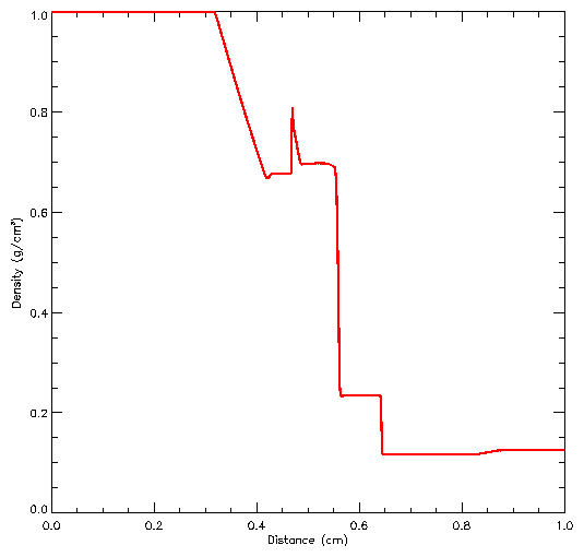
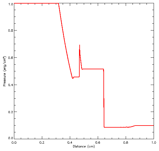
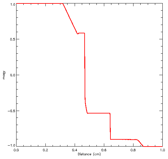
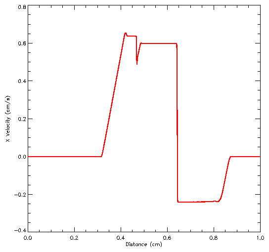
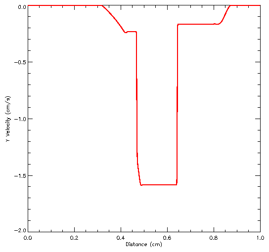
The linear instability of self-gravitating fluids was first explored by Jeans (1902) in connection with the problem of star formation. The nonlinear phase of the instability is of greatest astrophysical interest nowadays, but the linear instability provides a very useful test of the coupling of gravity to hydrodynamics in FLASH.

The jeans problem allows one to examine the behavior of sinusoidal, adiabatic density perturbations in both the pressure-dominated and gravity-dominated limits. This problem uses periodic boundary conditions. The equation of state is that of a perfect gas. The initial conditions at t=0 are

r(x) = r0[ 1 + d cos(k·x)] p(x) = p0[ 1 + gd cos(k·x)] (143) v(x) = 0 ,

where the perturbation amplitude d << 1. The stability of the perturbation is determined by the relationship between the wavenumber k º |k| and the Jeans wavenumber k_J, where k_J is given by

kJ º Ö 4pGr0 c0  ,

(144)

and where c₀ is the unperturbed sound speed:

c0 =   æ Ö  gp0 r0

(145)

(Chandrasekhar 1961). If k > k_J, the perturbation is stable and oscillates with frequency

w = Ö   c02k2 - 4pGr0    ;

(146)

otherwise it grows exponentially, with a characteristic timescale given by t = (iw)^-1.

We checked the dispersion relation (146) for stable perturbations with g = 5/3 by fixing r₀ and p₀ and performing several runs with different k. We followed each case for roughly five oscillation periods using a uniform grid in the box [0,L]². We used r₀ = 1.5×10⁷ g cm^-3 and p₀ = 1.5×10⁷ dyn cm^-2, yielding k_J = 2.747 cm^-1. The perturbation amplitude d was fixed at 10^-3. The box size L is chosen so that k_J is smaller than the smallest nonzero wavenumber which can be resolved on the grid:

L =  1 2   æ Ö  pgp0 Gr02    .

(147)

This prevents roundoff errors at wavenumbers less than k_J from being amplified by the physical Jeans instability. We used wavevectors k parallel to and at 45 degrees to the x-axis. Each test calculation used the multigrid Poisson solver together with its default settings.

The resulting kinetic, thermal, and potential energies as functions of time for one choice of k are shown in Figure 30 together with the analytic solution, which is given in two dimensions by

T(t) =  r0d2|w|2L2 8k2 [1-cos(2wt) ] U(t)-U(0) = -  1 8 r0c02d2L2[1-cos(2wt) ] (148) W(t) = -  pGr02d2L2 2k2 [1+cos(2wt) ] . (149)

The figure shows that FLASH obtains the correct amplitude and frequency of oscillation in this case. We computed the average oscillation frequency for each run by measuring the time interval required for the kinetic energy to undergo exactly ten oscillations. Figure 31 compares the resulting dispersion relation to equation (146). It can be seen from this plot that FLASH correctly reproduces equation (146). At the highest wavenumber (k = 100), each oscillation is resolved using only about 14 zones on a six-level uniform grid, and the average timestep (which depends on c₀, Dx, and Dy, and has nothing to do with k) turns out to be comparable to the oscillation period. Hence the frequency determined from the numerical solution for this value of k is somewhat more poorly determined than for the other runs. At lower wavenumbers, however, the frequencies are correct to less than 1%.

Figure 30: Kinetic, internal, and potential energy versus time for a stable Jeans mode with k=10.984. Points indicate numerical values found using FLASH 2.0 with a four-level uniform grid. The analytic solution for each form of energy is shown using a solid line.

Figure 31: Computed versus expected Jeans dispersion relation (for stable modes) found using FLASH 1.62 with a six-level uniform grid.

The additional runtime parameters supplied with the jeans problem are listed in Table 35. This problem is configured to use the perfect-gas equation of state (gamma), and it is run in a two-dimensional unit box with gamma set to 1.67. The refinement marking routine (ref_marking.F90) supplied with this problem refines blocks whose mean density exceeds a given threshold. Since the problem is not spherically symmetric, the multigrid Poisson solver should be used.

Table 40: Runtime parameters used with the jeans test problem.

Variable	Type	Default	Description
rho0	real	1	Initial unperturbed density (r0)
p0	real	1	Initial unperturbed pressure (p0)
amplitude	real	0.01	Perturbation amplitude (d)
lambdax	real	1	Perturbation wavelength in x direction (lx = 2p/kx)
lambday	real	1	Perturbation wavelength in y direction (ly = 2p/ky)
lambdaz	real	1	Perturbation wavelength in z direction (lz = 2p/kz)
delta_ref	real	0.1	Refine a block if the maximum density contrast relative to rref is greater than this
delta_deref	real	0.1	Derefine a block if the maximum density contrast relative to rref is less than this
reference_density	real	1	Reference density for grid refinement (rref). Density contrast is used to determine which blocks to refine; it is defined as max block  ì í î ê ê  rijk rref -1 ê ê ü ý þ	(150)

12.4.2  The homologous dust collapse problem

The homologous dust collapse problem is used to test the ability of the code to solve self-gravitating problems in which the flow geometry is spherical and gas pressure is negligible. The problem was first described by Colgate and White (1966) and has been used by Mönchmeyer and Müller (1989) to test hydrodynamical schemes in curvilinear coordinates. As the Poisson solvers currently included with FLASH do not yet work in curvilinear coordinates, we solve this problem using a 3D Cartesian grid.

The initial conditions consist of a uniform sphere of radius r₀ and density r₀ at rest. The pressure p₀ is taken to be constant and very small:

p0 <<  4pG g r02 r02 .

(151)

We refer to such a nearly pressureless fluid as `dust'. A perfect-gas equation of state is used, but the value of g is not significant. Outflow boundary conditions are used for the gas, while isolated boundary conditions are used for the gravitational field.

The collapse of the dust sphere is self-similar; the cloud should remain spherical and uniform as it collapses. The radius of the cloud, r(t), should satisfy

æ è  8pG 3 r0 ö ø 1/2   t = æ è 1-  r(t) r0 ö ø 1/2   æ è  r(t) r0 ö ø 1/2   +sin-1 æ è 1-  r(t) r0 ö ø 1/2

(152)

(Colgate & White 1966). Thus we expect to test three things with this problem: the ability of the code to maintain spherical symmetry during an implosion (in particular, no block boundary effects should be evident); the ability of the code to keep the density profile constant within the cloud; and the ability of the code to obtain the correct collapse factor. The second of these is particularly difficult, because the edge of the cloud is very sharp and because the Cartesian grid breaks spherical symmetry most dramatically at the center of the cloud, which is where all of the matter ultimately ends up.

Results of a dust_coll run using FLASH 1.62 appear in Figure 32. This run used 4³ top-level blocks and seven levels of refinement, for an effective resolution of 2048³ at the center of the grid. The multipole Poisson solver was used with a maximum multipole moment l = 0. The initial conditions used r₀ = 10⁹ g cm^-3 and r₀ = 6.5×10⁸ cm. In Figure 32a, the density, pressure, and velocity are scaled by 2.43×10⁹ g cm^-3, 2.08×10¹⁷ dyn cm^-2, and 7.30×10⁹ cm s^-1, respectively. In Figure 32b they are scaled by 1.96×10¹¹ g cm^-3, 2.08×10¹⁷ dyn cm^-2, and 2.90×10¹⁰ cm s^-1. Note that within the cloud the profiles are very isotropic, as indicated by the small dispersion in each profile. Significant anisotropy is only present for `fluff' material flowing in through the Cartesian boundaries. In particular, it is encouraging that the velocity field remains isotropic all the way into the center of the grid; this shows the usefulness of refining spherically symmetric problems near r=0. However, as material flows inward past refinement boundaries, small ripples develop in the density profile due to interpolation errors. These remain spherically symmetric but increase in amplitude as they are compressed. Nevertheless, they are still only a few percent in relative magnitude by the second frame. The other numerical effect of note is a slight spreading at the edge of the cloud. This does not appear to worsen significantly with time. If one takes the radius at which the density drops to one-half its central value as the radius of the cloud, then the observed collapse factor agrees with our expectation from equation (152). Overall our results, including the numerical effects, agree well with those of Mönchmeyer and Müller (1989).

The additional runtime parameters supplied with the dust_coll problem are listed in Table 36. This problem is configured to use the perfect-gas equation of state (gamma), and it is run in a three-dimensional box with gamma set to 1.67. The refinement marking routine (ref_marking.F90) supplied with this problem refines blocks containing the center of the cloud. Since the problem is spherically symmetric, either the multigrid or multipole solvers can be used.

Figure 32: Density (black), pressure (red), and velocity (blue) profiles in the homologous dust collapse problem at (a) t=0.0368 sec and (b) t=0.0637 sec. The density, pressure, and velocity are scaled as discussed in the text.

Table 41: Runtime parameters used with the dust_coll test problem.

Variable	Type	Default	Description
rho0	real	1	Initial cloud density (r0)
R_init	real	0.05	Initial cloud radius (r0)
T_ambient	real	1	Initial ambient temperature
xctr	real	0.5	x-coordinate of cloud center
yctr	real	0.5	y-coordinate of cloud center
zctr	real	0.5	z-coordinate of cloud center

12.4.3  The Huang-Greengard Poisson test problem

The poistest problem tests the convergence properties of the multigrid Poisson solver on a multidimensional, highly (locally) refined grid. This problem is described by Huang and Greengard (2000). The source function consists of a sum of thirteen two-dimensional Gaussians:

r(x,y) = 13 å i=1  e-si[(x-xi)2+(y-yi)2] ,

(153)

where the constants s_i, x_i, and y_i are given in Table 37. The very large range of widths and ellipticities of these peaks forces the mesh structure to be highly refined in some places. The density field and block structure are shown for a 14-level mesh in Figure 33.

Figure 33: Density field and block structure for a 14-level mesh applied to the Huang-Greengard test problem. The effective resolution of the mesh is 65,536².

Table 42: Constants used in the poistest problem.

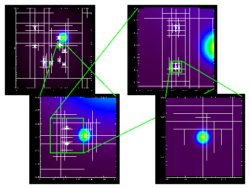
i	1	2	3	4	5	6	7
xi	0	-1	-1	0.28125	0.5	0.3046875	0.3046875
yi	0	0.09375	1	0.53125	0.53125	0.1875	0.125
si	0.01	4000	20000	80000	16	360000	400000
i	8	9	10	11	12	13
xi	0.375	0.5625	-0.5	-0.125	0.296875	0.5234375
yi	0.15625	-0.125	-0.703125	-0.703125	-0.609375	-0.78125
si	2000	18200	128	49000	37000	18900

The poistest problem uses no additional runtime parameters beyond those required by the rest of the code.

12.5  Other test problems

12.5.1  The sample_map problem

Frequently when doing simulations, one needs to initialize the computational domain with a one-dimensional model from a stellar evolution (or other) code. A simple framework for accomplishing this task is provided by the sample_map problem. This is intended to be a template for users to modify to suit their needs.

This problem is composed of two main routines, init_1d and the familiar init_block. init_1d reads the initial model from disk, determines which variables are present and how they map into the variables defined in FLASH, and stores the initial model in arrays that are then used by init_block. The general format of an initial model file is a single comment line, a line giving the number of variables contained in the initial model, the 4-character names of each variable (one per line), followed by the data (spatial coordinate first), with the variables in the same order as the list of names. An example of this format follows.

 
# sample 1-d model
number of variables = 7
dens
pres
ener
gamc
game
fuel
ash
0.01 10. 100. 25. 1.4 1.4 1.0 0.0
0.02 9.5. 95. 25. 1.4 1.4 0.99 0.0
:

In the above sample file, we define seven variables. The first zone starts with the coordinate of the zone center (0.01) and then lists the density (10.), pressure (100.), and so forth, with one entry for each variable per line. The next zone of the initial model is listed immediately below this line. init_1d will continue to read in zones for the initial model until it encounters the end of the file.

FLASH contains more variables than the seven defined in this input file, and it will initialize any variables not specified in the input file to zero. Additionally, sometimes a variable is specified in the input file, but there is no corresponding variable defined in FLASH. In this case, init_1d will produce a warning, listing the variables it does not know about. Finally, there is no need for the variables to be listed in the same order as they are stored in the FLASH data structures-they will be sorted as each zone is read from the initial model.

The inital model is stored in two data structures: xzn(N1D_MAX) contains the coordinates of the initial model zone centers, and model_1d(N1D_MAX, nvar) contains the values of the variables defined in the initial model. These are stored in the same order as the variables in the solution array unk maintained by FLASH. N1D_MAX is a parameter specifying the maximum number of zones in the initial model (currently set to 2048).

These data structures are passed to the init_block function which loops over all of the zones in the current block, determines the x-, y-, and z-coordinates of the zone, and performs an interpolation to find the values of the initial variables in the current zone. This interpolation attempt to construct as zone average from the values of the initial model at the zone edges and center.

There are two parameters for this problem, model_file is a string that gives the name of the input file to read the initial model from. imap_dir is an integer the specifies the direction to map the initial model along, imap_dir = 1 maps along the x-direction, 2 maps along the y direction, and 0 maps it in a circle in the x-y plane.

Part 5
TOOLS

13  The FLASH configuration script (setup)

The setup script, found in the FLASH root directory, provides the primary command-line interface to the FLASH source code. It configures the source tree for a given problem and target machine and creates files needed to parse the runtime parameter file and make the FLASH executable. More description of what setup does may be found in Section 3. Here we describe its basic usage.

Running setup without any options prints a message describing the available options:

[sphere 5:09pm] % ./setup
usage: setup <problem-name> [options]

              problems: see /home/user/FLASH2.0/setups/
              options: -verbose -portable -auto -[123]d -maxblocks=<#>
                           [-site=<site> | -ostype=<ostype>] [-debug | -test]                            -preprocess -report -objdir=<relative obj directory>

For compatibility with older versions of setup, the syntax

              setup <problem-name> <ostype> [options]

is also accepted, so long as <ostype> does not begin with a dash (-). In this case the -site and -ostype options cannot be used. Available values for the mandatory option (the name of the problem to configure) are determined by scanning the setups/ directory.

A ``problem'' consists of a set of initial and boundary conditions, possibly additional physics (e.g., a subgrid model for star formation), and a set of adjustable parameters. The directory associated with a problem contains source code files which implement the initial conditions and, in a few cases, the boundary conditions and extra physics, together with a configuration file, read by setup, which contains information on required physics modules and adjustable parameters.

setup determines site-dependent configuration information by looking in source/sites/ for a directory with the same name as the output of the hostname command; failing this, it looks in source/sites/Prototypes/ for a directory with the same name as the output of the uname command. The site and operating system type can be overridden with the -site and -ostype command-line options. Only one of these options can be used. The directory for each site or operating system type contains a makefile fragment ( Makefile.h) that sets command names, compiler flags, and library paths, and any replacement or additional source files needed to compile FLASH for that machine type.

setup uses the problem and site/OS type, together with a user-supplied file called Modules which lists the code modules to include, to generate a directory called object/ which contains links to the appropriate source files and makefile fragments. It also creates the master makefile (object/Makefile) and several Fortran include files that are needed by the code in order to parse the runtime parameter file. After running setup, the user can make the FLASH executable by running gmake in the object/ directory (or from the FLASH root directory, if the -portable option is not used with setup). The optional command-line modifiers have the following interpretations:

-verbose	Normally setup echoes to the standard output summary messages indicating what it is doing. Including the -verbose option causes it to also list the links it creates.
-portable	This option creates a portable build directory. Instead of object/, setup creates object_problem/, and it copies instead of linking to the source files in source/ and setups/. The resulting build directory can be placed into a tar archive and sent to another machine for building (use the Makefile created by setup in the tar file).
-auto	This modifier replaces -defaults, which is still present in the code but has been deprecated. Normally setup requires that the user supply a plain text file called Modules (in the FLASH root directory) which specifies which code modules to include. A sample Modules file appears in Figure 34. Each line is either a comment (preceded by a hash mark (#)) or a module include statement of the form INCLUDE module. Sub-modules are indicated by specifying the path to the sub-module in question; in the example, the sub-module gamma of the eos module is included. If a module has a default sub-module, but no sub-module is specified, setup automatically selects the default using the module's configuration file.
	The -auto option enables setup to generate a ``rough draft'' of a Modules file for the user. The configuration file for each problem setup specifies a number of code module requirements; for example, a problem may require the perfect-gas equation of state (materials/eos/gamma) and an unspecified hydro solver (hydro). With -auto, setup creates a Modules file by converting these requirements into module include statements. In addition, it checks the configuration files for the required modules and includes any of their required modules, eliminating duplicates. Most users configuring a problem for the first time will want to run setup with -auto to generate a Modules file, then edit Modules directly to specify different sub-modules. After editing Modules in this way, re-run setup without -auto to incorporate the changes into the code configuration.
-[123]d	By default setup creates a makefile which produces a FLASH executable capable of solving two-dimensional problems (equivalent to -2d). To generate a makefile with options appropriate to three-dimensional problems, use -3d. To generate a one-dimensional code, use -1d. These options are mutually exclusive and cause setup to add the appropriate compilation option to the makefile it generates.
-maxblocks=#	This option is also used by setup in constructing the makefile compiler options. It determines the amount of memory allocated at runtime to the adaptive mesh refinement (AMR) block data structure. For example, to allocate enough memory on each processor for 500 blocks, use -maxblocks=500. If the default block buffer size is too large for your system, you may wish to try a smaller number here (the defaults are currently defined in source/driver/physicaldata.fh). Alternatively, you may wish to experiment with larger buffer sizes if your system has enough memory.
-debug	The default Makefile built by setup will use the optimized setting for compilation and linking. Using -debug will force setup to use the flags relevant for debugging (e.g., including -g in the compilation line).
-test	When FLASH is tested by the automated test suite, test will choose the paper compilation arguments for the test executable.
-preprocess	This option will preprocess all of the files before compilation. This is useful for machines whose compilers do not support preprocessing.
-report	For setup to list all of the modules used by the current configuration.
-objdir	Overrides the default object directory with one whose name is specified by this parameter.

When setup is run, it reads all of the Config files in the module directories to find the runtime parameters that the code understands. Two files are created by setup that list the available runtime parameters, paramFile.txt and paramFile.html. These files contain a list of all of the runtime parameters that are understood by FLASH and some brief comments describing their purpose, both in text ((ASC)I) and HTML format. In addition to the name, comments (if available), the default value, and the module that owns the parameter. These files provide a useful way to determine which parameters can be used in a flash.par for a given problem.

# Modules file constructed for rt problem by setup -auto INCLUDE driver/time_dep INCLUDE hydro INCLUDE materials/eos/gamma INCLUDE gravity/constant INCLUDE mesh INCLUDE io

Figure 34: Example of the Modules file used by setup to determine which code modules to include.

To set runtime parameters to values other than the defaults, create a runtime parameter file named flash.par in the directory from which FLASH is to be run. The format of this file is described briefly in Section , and in more detail in Section 16.3.

Setup also creates two functions that are used by FLASH. buildstamp takes a file logical unit number and outputs the date and time the current FLASH executable was setup, along with the platform information. flash_release returns a character string containing the full version number (including the minor version number) of the present build of FLASH.

14  sfocu (Serial Flash Output Comparison Utility)

sfocu is intended as a replacement for focu (available in previous versions of FLASH) and is mainly used as part of an automated testing suite called flash_test.

sfocu is a serial utility which examines two FLASH checkpoint files and decides whether or not they are ``equal'' to ensure that any changes made to FLASH do not adversely affect subsequent simulation output. By ``equal,'' we mean that:

• The leaf-block structure matches: each leaf block must have the same position and size in both datasets.
• The data arrays in the leaf blocks (dens, pres...) are identical.

Thus, sfocu ignores information such as the particular numbering of the blocks, the timestamp, the build information, and so on.

sfocu can read both HDF4 and HDF5 FLASH checkpoint files. It does not support f77 checkpoint files, and has not been tested with FLASH checkpoints that span multiple files. Although sfocu is a serial program, it is able to do comparisons on the output of large parallel simulations. sfocu has been used on irix, linux, AIX and OSF1.

14.1  Building sfocu

The process is entirely manual, although Makefiles for certain machines have been provided. There are a few compile-time options which you set via the following preprocessor definitions in the Makefile:

NO_HDF4

build without HDF4 support

NO_HDF5

build without HDF5 support

SHORT_REPORT

produce a more concise report that fits better on a standard terminal

NEED_MPI

certain parallel versions of HDF5 need to be linked with the MPI library. This adds the necessary MPI_Init, MPI_Finalize calls to sfocu. There is no advantage to running sfocu on more than one processor, it will only give you multiple copies of the same report.

14.2  Using sfocu

There are no command line options. Simply run the command sfocu <file1> <file2>. Sample output follows:

Comparing:      a/windtunnel_4lev_hdf_chk_0001
                b/windtunnel_4lev_hdf_chk_0001

Norm used:      d(a,b) = abs(2(a-b)) / max(abs(a+b), 1e-99)

Total leaf blocks compared: 1032

Var     Bad Blocks      Min Error       Max Error
===================================================
pres    868             0               6.59229e-11
temp    880             0               1.95468e-10
gamc    0               0               0
dens    867             0               5.98321e-11
velx    866             0               1.87844e-11
vely    1032            0               2773.88
velz    0               0               0
ener    867             0               3.41799e-11
game    0               0               0
 1      885             0               1.95472e-10
FAILURE

"Bad Blocks" is the number of leaf blocks where the data was found to differ between datasets; "Min Error" and "Max Error" are the minimum and maximum of the norm defined in the output. The last line makes it easier for other programs to parse sfocu output: when the files are identical, the line will instead read SUCCESS.

If the SHORT_REPORT compile-time option isn't used, sfocu will also report the maximum, minimum and sum of the variables in the two files, to give you an idea of the scales involved. Note that the error norm is dimensionless.

It's possible for sfocu to miss machine-precision variations in the data on certain machines because of compiler or library issues. Or possibly even bugs (!). This has only been observed on one platform, where the compiler produced code that ignored IEEE rules until the right flag was found.

15  FLASH IDL routines (fidlr)

fidlr is a set of routines, written in the IDL, that can plot or read data files produced by FLASH. The routines include programs which can be run from the IDL command line to read 1D, 2D, or 3D FLASH datasets, interactively analyze datasets, and interpolate them onto uniform grids. Other IDL programs (xflash and cousins) provide a graphical interface to these routines, enabling users to read and plot AMR datasets.

Currently, the fidlr routines support 1, 2, and 3-dimensional datasets in the FLASH HDF or HDF5 formats. Both plotfiles and checkpoint files are supported, as they differ only in the number of variables stored, and possibly the numerical precision. Since IDL does not directly support HDF5, the call_external function is used to interface with a set of C routines that read in the HDF5 data (see section 5). Using these routines requires that the HDF5 library be installed on your system and that the shared-object library be compiled before reading in data. Since the call_external function is used, the demo version of IDL will not run the routines.

For basic plotting operations, the easiest way to generate plots of FLASH data is to use one of the widget interfaces: xflash1d for 1d data, xflash for 2d data, and xflash3d for 3d data. For more advanced analysis, the read routines can be used to read the data into IDL, and it can then be accessed through the common blocks. Examples of using the fidlr routines from the command line are provided in § 15.6. Additionally, some scripts demonstrating how to analyze FLASH data using the fidlr routines are described in Section 15.5 (see for example radial.pro).

The driver routines provided with fidlr visualize the AMR data by first converting it to a uniform mesh. This allows for ease of plotting and manipulation, including contour plotting, but it is less efficient than plotting the native AMR structure. Analysis can still be performed directly on the native data through the command line.

15.1  Installing and running fidlr

fidlr is distributed with FLASH and contained in the tools/fidlr/ directory. In addition to the IDL procedures, a README file is present which will contain up-to-date information on changes and installation requirements.

These routines were written and tested using IDL v5.3 for IRIX. They should work without difficulty on any UNIX machine with IDL installed-any functionality of fidlr under Windows is purely coincidental. Later versions of IDL no longer support GIF files due to copyright difficulties, so outputting to a image file may not work. At present, we do not have access to this version, but it should be possible to replace the GIF functionality with PNG images. It is possible to run IDL in a `demo' mode if there are not enough licenses available. Unfortunately, some parts of fidlr will not function in this mode, as certain features of IDL are disabled. This guide assumes that you are running the full version of IDL.

Installation of fidlr requires defining some environment variables, and compiling the support for HDF5 files. These procedures are described below.

15.1.1  Setting up fidlr environment variables

The FLASH IDL routines are located in the tools/fidlr/ subdirectory of the FLASH root directory. To use them you must set two environment variables. First set the value of XFLASH_DIR to the location of the FLASH IDL routines; for example, under csh, use

setenv XFLASH_DIR flash-root-path/tools/fidlr

where flash-root-path is the absolute path of the FLASH root directory. This variable is used in the plotting routines to find the customized color table for xflash, as well as to identify the location of the shared-object libraries compiled for HDF5 support.

Next, make sure you have an IDL_DIR environment variable set. Ths should point to directory in which the IDL distribution is installed. For example, if IDL is installed in idl-root-path, then you would define:

setenv IDL_DIR idl-root-path

Finally, you need to tell IDL where to find the fidlr routines. This is accomplished through the IDL_PATH environment variable:

setenv IDL_PATH ${XFLASH_DIR}:${IDL_DIR}:${IDL_DIR}/lib

If you already have an IDL_PATH environment variable defined, just add XFLASH_DIR to the beginning of it. You may wish to include these commands in your .cshrc or .profile file (depending on your shell) to avoid having to reissue them every time you log in.

15.1.2  Setting up the HDF5 routines

For fidlr to read HDF5 files, you need to install the HDF5 library on your machine and compile the wrapper routines. The HDF5 libraries can be obtained in either source or binary form for most Unix platforms from http://hdf.ncsa.uiuc.edu. The Makefile with fidlr supplied will create the shared-object library on an SGI, but will need to be edited for other platforms. The compiler flags for a shared-object library for different versions of Unix can be found in

${IDL_DIR}/external/call_external/C/callext_unix.txt

The compilation flags in the Makefile should be modified according to the instructions in that file. Additionally, the Makefile needs to know where the HDF5 library is installed as well. This is set through the HDF5path definition in the Makefile.

It is important that you compile the shared-object to conform to the same application binary interface (ABI) that IDL was compiled with. On an SGI, IDL version 5.2.1 and later use the n32 ABI, while versions before this are o32. The HDF library will also need to be compiled in the same format. You can check the format of the HDF5 library and your version of IDL with the UNIX file command.

IDL interacts with external programs through the call_external function. Any arguments are passed by reference through the standard C command line argument interface, argc and argv. These are recast into pointers of the proper type in the C routines. The C wrappers call the appropriate HDF functions to read the data and return it through the argc pointers.

15.1.3  Running IDL

fidlr uses 8-bit color tables for all of its plotting. On displays with higher color depths, it may be necessary to use color overlays to get the proper colors on your display. For SGI machines, launching IDL with the start.pro script with enable 8-bit pseudocolor overlays. For Linux boxes, setting the X color depth to 24-bits per pixel and launching IDL with the start_linux.pro script usually produces proper colors.

15.2  fidlr data structures

The fidlr routines access the data contained in the FLASH output files through a series of common blocks. For the most part, the variable names are consistent with the names used in FLASH. It is assumed that the user is familiar with the block structured AMR format employed by FLASH (refer to § 5 for full details of the output format). All of the unknowns are stored together in the unk data structure, which mirrors that contained in FLASH itself. The list of variable names is contained in the string array unk_names. A utility function var_index is provided to convert between a 4-character string name and the index into unk. For example,

unk[var_index('dens'),*,*,*,*]

selects the density from the unk array. Recall that IDL uses zero-based indexing for arrays.

fidlr will attempt to create derived variables from the variables stored in the output file if it can. For example, the total velocity can be created from the components of the velocity, if they are all present. A separate data structure varnames contains the list of variables in the output file plus any additional variables fidlr knows how to derive.

At present, the global common blocks defined by fidlr are:

common size, tot_blocks, nvar, nxb, nyb, nzb, ntopx, ntopy, ntopz
common time, time, dt
common tree, lrefine, nodetype, gid, coord, size, bnd_box
common vars, unk, unk_names
common particles, numParticles, particles

These can be defined on the command line by executing the def_common script provided in the fidlr directory. This allows for analysis of the FLASH data through the command line with any of IDLs built in functions. For example, to find the minimum density in the leaf blocks of the file filename_hdf_chk_0000, you could execute:

IDL> .run def_common
IDL> read_amr, 'filename_hdf_chk_0000'
IDL> leaf_blocks = where(nodetype EQ 1)
IDL> print, min(unk[var_index('dens'),*,*,*,leaf_blocks])

Here, in addition to the unk data-structure, we used the nodetype array, which is set to 1 if a block is a leaf (as it is in FLASH).

15.3  xflash: plotting two-dimensional datasets

The main interface to the fidlr routines for plotting 2-dimensional data sets is xflash. xflash produces colormap plots of FLASH data with optional velocity vectors, contours, and the AMR block structure overlaid. The basic operation of xflash is to specify a file or range of files, probe the file for the list of variables it contains (through the discover variables button described below), and then specify the remaining plot options.

xflash can output to the screen, postscript, or an image file (GIF). If the data is significantly higher resolution than the output device, then xflash (through xplot_amr.pro) will sub-sample the image by one or more levels of refinement before plotting.

Once the image is plotted, the query button will become active. Pressing query and then clicking anywhere in the domain will pop up a window containing the values of all the FLASH variables in the zone nearest the cursor. The query function uses the actual FLASH data-not the interpolated/uniformy gridded data generated for the plots

Figure 35: The main xflash widget (a) and the widget showing the variable list dropbox (b).

Typing xflash at the IDL command prompt will launch the main xflash widget, shown in Figure 35(a). The widget is broken into several sections, with some features initially disabled. These sections are explained below.

 
File Options

The file to be visualized is composed of the path, the basename (the same base name used in the flash.par) plus any file type information appended to it (ex. 'hdf_chk_') and the range of suffices to loop through. An optional parameter, step, controls how many files to skip when looping over the files. By default, xflash sets the path to the working directory that IDL was started from. xflash will spawn gzip if the file is stored on disk compressed and the file is gzipped box is checked. After the file is read, it will be compressed again.

Once the file options are set, clicking on discover variables will read the variable list from the first file specified, and use the variable names to populate the variable selection box. xflash will automatically determine if the file is an HDF or HDF5 file, and read the `unknown names' record to get the variable list. This will work for both plotfiles and checkpoint files generated by FLASH.

 
Output Options

A plot can be output to the screen (default), a Postscript file, or a GIF file. The output filenames are composed from the basename + variable name + suffix. For outputs to the screen or GIF, the plot size options allow you to specify the image size in pixels. For Postscript output, xflash chooses portrait or landscape orientation depending on the aspect ratio of the domain.

 
Problem

The problem dropbox allows you to select one of the predefined problem defaults. This is provided soley for convienence, as users frequently want to plot the same problem using the same data ranges. This will load the options (data ranges, velocity parameters, and contour options) for the problem as specified in the xflash_defaults procedure. When xflash is started, xflash_defaults is executed to read in the known problem names. The data ranges and velocity defaults are then updated. To add a problem to xflash, only the xflash_defaults procedure needs to be modified. The details of this procedure are provided in the comment header in xflash_defaults. It is not necessary to add a problem in order to plot a dataset, as all default values can be overridden through the widget.

 
Variables

The variables dropbox lists the variables stored in the `unknown names' record in the data file, and any derived variables that xflash knows how to construct from these variables (ex: sound speed). This allows you to choose the variable to be plotted. By default, xflash reads all the variables in a file, so switching the variable to plot can be done without rereading. At present, there is no easy way to add a derived variable. Both the widget routine ( xflash.pro) and the plotting backend (xplot_amr.pro) will need to be told about any new derived variables. Users wishing to add derived variables should look at how the total velocity ( tot_vel) is computed.

 
Colormap

The colormap dropbox lists the available colormaps to xflash. These colormaps are stored in flash_colors.tbl in the fidlr directory, and differ from the standard IDL colormaps. The first 12 colors in the colormaps are reserved by xflash to hold the primary colors used for different aspects of the plotting. Additional colormaps can be created by using the xpalette function in IDL. It is suggested that new colormaps use one of the existing colormaps as a template, to preserve the primary FLASH colors.

 
Options

The options block allows you to toggle various options on/off (Table 39).

Table 43: xflash options
log	Plot the log of the variable.
max	When looping over a sequence of files, plot the max of the variable in each zone over all the files.
annotate	Toggle the title and time information.
abs value	Plot the absolute value of the dataset. This operation is performed before taking the log.
show blocks	Draw the block boundaries on the plot.
colorbar	Plot the colorbar legend for the data range.
show ticks	Show the axis/tick marks on the plot.

 
 
Data Range

These fields allow you to specify the range of the variable to plot. Data outside of the range will be scaled to the minimum and maximum values of the colormap respectively.

 
Contour Options

This launches a dialog box that allows you to select up to 4 contour lines to overplot of the data (see figure 36). The variable, value, and color are specified for each reference contour. To plot a contour, select the check box next to the contour number. This will allow you to set the variable to make the contour from, the value of the contour, and the color.

Figure 36: The xflash contour option subwidget.

 
Velocity Options

This launches a dialog box that allows you to set the velocity options used to plot velocity vectors on the plot (see figure 37). The plotting of velocity vectors is controlled by the partvelvec.pro procedure. xskip and yskip allow you to thin out the arrows. typical velocity sets the velocity to scale the vectors to, and minimum velocity and maximum velocity specify the range of velocities to plot vectors for.

Figure 37: The xflash velocity option subwidget.

 
Particle Options

If a FLASH output file contains particle data, the particle options button will be made sensitive. This button launches a dialog box that allows you to set the particle options used to plot the particles a plot (see figure 38). The plotting of particles vectors is controlled by the partvelvec.pro procedure. The position of a particle is marked with a circle, whose size can be controlled by the symbol size slider. The typical velocity field allows you to adjust the scaling of the particle velocity vectors.

Figure 38: The xflash particle option subwidget.

 
Zoom

The zoom options allow you to set the domain limits for the plot. A value of -1 uses the actual limit of the domain.

 
Plot

Create the plot. The status of the plot will appear on the status bar at the bottom.

 
Query

The query button becomes active once the plot is created. Clicking on query and then clicking somewhere in the domain lists the data values at the cursor location (see Figure 39).

Figure 39: The xflash query widget, displaying information for a zone.

15.4  xflash3d: plotting slices of three-dimensional datasets

xflash3d provides an interface for plotting slices of 3-dimension FLASH datasets. It is written to conserve memory-only a single variable is read in at a time, and only the slice to be plotted is put on a uniform grid. The merging of the AMR data to a uniform grid is accomplished by merge3d_amr.pro which can take a variety of arguments which control what volume of the domain is to be put onto a uniform grid.

Figure 40: The xflash3d widget.

Figure 40 shows the main xflash3d widget. The interface is similar to that of xflash, so the above description from that section still applies. The major difference is in the zoom section, which controls the slice plane.

The slice plane button group controls the plane to plot the data in. For a given plane, the direction orthogonal will have only on active text box to enter zoom information-this controls the position of the slice plane in the normal direction. For the directions in the slice plane, the zoom boxes allow you to select a sub-domain in that plane to plot.

15.5   The fidlr routines

Table 40 lists all of the fidlr routines, grouped by function. Most of these routines rely on the common blocks to get the tree structure necessary to interpret a FLASH dataset. Command line analysis of FLASH data requires that the common blocks be defined, usually by executing def_common.pro.

Table 44: Description of the fidlr routines
Table 45: fidlr routines-continued
FLASH data readers
read_amr.pro	Read in FLASH data in HDF 4 format. This routine takes the filename and an optional variable argument and returns then tree, grid, and unknown information in the fidlr  common blocks.
read_amr_hdf5.pro	The HDF5 version of read_amr.pro. This routine uses the call_external function to access C wrappers of the HDF functions stored in h5_wrappers.so. The shared library must be compiled before using this routine.
file_information.pro	Dump out some basic information about the file, such as the number of variables store, the runtime comment, the precision of the data, etc.
Driver routines
xflash.pro	The main driver for 2d datasets. xflash provides a widget interface to select the variable, data range, contour options, output type, etc. This routine uses xflash_defaults.pro to define some default problem types and their options. Once the options are selected, xplot_amr.pro is used to create the plot.
xflash1d.pro	The main driver for 1d datasets. This widget accepts options and passes them onto xplot1d_amr.pro.
xflash3d.pro	The main driver for 3d datasets. This widget allows you to select the cut plane (x-y, x-z, y-z) and set the data options. xplot3d_amr.pro is used to create the plots.
xflash_defaults.pro	The problem default initialization file. Standard problems are given an entry in this file, defining the default values for the plot options. This file is read in by xflash, xflash1d, and xflash3d when the problem name is changed.
xcontour.pro	The contour options widget. This allows you to select up to 4 reference contours to be overplotted on a 2d plot. This widget is launched by xflash.pro.
xvelocity.pro	The velocity options widget. This allows you to select the minimum, maximum, and typical velocities, and the number of zones to skip when thinning out the vector field. This widget is launched by xflash.pro.
xparticle.pro	The particle options widget. This widget is launched by xflash.pro.
batch.pro	An example script showing how to convert a 3d FLASH dataset to a uniformly gridded single byte block of data suitable for 3d visualization packages. The block of data is written in Fortran binary format.
radial.pro	An example script showing how to read in 2d data and plot a variable as a function of radius from a given point.
compare.pro	A script showing how to loop over a set of files and plot a series of 1d slices of a variable vs distance.
flame_profile.pro	A script that reads in a 2-d FLASH dataset and writes out a 1d slice of data to an (ASC)I file.
flame_profile_1d.pro	A script that reads in a 1-d FLASH dataset and writes out a 1d slice of data to an (ASC)I file. The format of the output file is identical to that required by the sample_map setup.
flame_speed.pro	Read in two FLASH files and compute the speed of a planar front by differencing.
HDF routines
hdf_read.pro	Wrapper around IDL HDF 4 routines to read in a dataset given the file handle and dataset name.
determine_file_type.pro	IDL procedure to determine if a file is in HDF 4 format (return 1), HDF5 format (return 2), or neither (return -1). This routine uses the built in IDL HDF 4 implementation and some of the HDF5 wrappers in h5_wrappers.so.
Makefile	Makefile for compiling the HDF5 support on an SGI IRIX. Other machines should behave similarly, but some of the compilation flags may differ.
h5_file_interface.c	HDF5 file open and close routines from the FLASH serial HDF5 implementation.
h5_read.c	Part of the serial HDF5 FLASH routines, used to read in the header information from the data file.
h5_wrappers.c	Wrappers around the HDF5 library to read in the different records from the FLASH HDF5 file.
h5_wrappers.so	Shared-object library produced from the above routines. The IDL routines interface with this object through the call external function.
hdf5_idl_interface.h	Header file for the C wrappers.
Merging routines
merge3d_amr.pro	Merge routine for 3d block structured AMR data. This routine will resample the FLASH data to put it on a uniform resolution. If the range keywords are used, a uniform slice can be created.
merge3d_amr_crn.pro	As above, but operates on data stored at the zone corners. This simply averages the data to the zone centers before proceeding.
merge_amr.pro	2d merging routine, put a dataset onto a uniform grid.
Plotting routines
draw_blocks.pro	Draw the AMR block boundaries on the plot. This routine is called from xflash.
vcolorbar.pro	Create a vertical colorbar given the data range and color bounds.
colorbar2.pro	Create a horizontal colorbar.
partvelvec.pro	Overplot the velocity vectors, for velocities that fall within a specified minimum and maximum velocity. The vectors are scaled to a typical velocity. This routine also handles the plotting of the particle data.
xplot1d_amr.pro	Back end to xflash1d-create a plot of a 1d FLASH dataset, using the options selected in the widget.
xplot3d_amr.pro	Back end to xflash3d-plot a slice through a 3d FLASH dataset.
xplot_amr.pro	Back end to xflash-plot a 2d dataset.
Utility routines
add_var.pro	add_var is used to add a derived variable to the list of variables recognized by the xflash  routines.
color.pro	color returns the index into the color table of a color specified by a string name.
color_gif.pro	Create a gif of the current plot window.
courant.pro	Loop over the blocks and return the block number where the Courant condition is set.
def_common.pro	Define the common blocks that hold the variables read in from the read routines. This routine can be used on the IDL command line so the FLASH data can be analyzed interactively.
flash_colors.tbl	Replacement color table with the standard FLASH colormaps.
nolabel.pro	A hack used to plot an axis w/o numbers.
query.pro	A widget routine called by xflash that displays the data in a cell of the current plot.
query1d.pro	Query routine for the 1d data, called from xflash1d.
scale3d_amr.pro	Scale a uniformly gridded 3d dataset into a single byte.
scale_color.pro	Scale a dataset into a single byte.
sci_notat.pro	Print a number out in scientific notation.
start.pro	A script used to initialize IDL on the SGIs.
tvimage.pro	Replacement for tv that will write to postscript or the screen in device independent manner.
undefine.pro	Free up the memory used by a variable.
var_index.pro	Return the index into the unk array of the variable label passed as an argument.
write_brick_f77.pro	Write a block of data out to a file in f77 binary format.

15.6  fidlr command line example

Most of the fidlr routines can be used directly from the command line to perform analysis not offered by the different widget interfaces. This section provides an example of using the fidlr routines.

 
Example. Report on the basic information about a FLASH data file.

IDL> file_information, 'sedov_2d_6lev_hdf_chk_0000'

-------------------------------------------------------------------------------
 file  = sedov_2d_6lev_hdf_chk_0000

 FLASH version:       FLASH 2.0.20010802
 file format:         HDF 4

 execution date:      08-03-2001  12:59.20
 run comment:         2D Sedov explosion, from t=0 with r_init = 3.5dx_min

 dimension:                  2
 geometry detected:   Cartesian (assumed)

 type of file:        checkpoint

 number of variables:           12
 variable precision:  DFNT_FLOAT64

 number of particles:        0

 nxb, nyb, nzb:                  8           8           1
 corners stored:      no

IDL>

Part 6
FURTHER DEVELOPMENT

16  Creating new problems

Every problem that is run with FLASH requires a directory in FLASH2.0/setups. This is where the FLASH setup script looks to find the problem-specific files. The FLASH distribution includes a number of pre-written setups. However, most new FLASH users will begin by defining a new problem, so it is important to understand the technique for adding a customized problem setup.

Each setups directory contains the routines that initialize the FLASH grid. The directory also includes parameter files that setup uses to select the proper physics modules from the FLASH source tree. When the user runs setup, the proper source files are selected and linked to the object directory (note here to refer to setup script docs).

There are two files that must be included in the setup directory for any problem. These are

Config	lists the modules required for the setup and defines additional runtime parameters.
init_block.F90	Fortran routine for setting initial conditions in a single block.

We will look in detail at these files for an example setup. This is a simple setup that creates a domain with hot ash inside a circle of radius radius centered at (xctr, yctr, zctr). The density is uniformly set at rho_ambient and the temperature is t_perturb inside the circle and t_ambient outside.

To create a new setup, we first create the new directory and then add the Config and init_block.F90 files. The easiest way to construct these files is to use files from another setup as a template.

16.1  Creating a Config file

The simplest way to construct a Config file is to copy one from another setup that incorporates the same physics as the new problem. Config serves two principal purposes: (1) to specify the required modules and (2) to register runtime parameters. The Config file for the example problem contains the following:

# configuration file for our example problem

REQUIRES driver/time_dep
REQUIRES materials/eos/gamma
REQUIRES materials/composition/fuel+ash
REQUIRES io
REQUIRES mesh
REQUIRES hydro

These lines define the FLASH modules used by the setup. We are going to carry wo fluids (fuel and ash), so we load the composition module fuel+ash. At runtime, this module will initialize the multifluid database to carry the two fluids, and it will setup their properties. We wish to rely on the defaults for I/O, meshing, and hydrodynamics, and select the simple gamma law eos ( materials/eos/gamma) for this problem.

Additional modules may be added to the Config file using this syntax. For example, to use the 13 isotope alpha-chain network, add the line:

REQUIRES source_terms/burn/aprox13

To add constant gravity, add the line:

REQUIRES gravity/constant

After defining the modules, the Config file lists any runtime parameters specific to this problem:

# runtime parameters
PARAMETER rho_ambient   REAL    1.
PARAMETER t_ambient     REAL    1.
PARAMETER t_perturb     REAL    5.
PARAMETER radius        REAL    0.2
PARAMETER xctr          REAL    0.5
PARAMETER yctr          REAL    0.5
PARAMETER zctr          REAL    0.5

Here we define the ambient density (rho_ambient), the ambient and perturbed temperatures (t_ambient, t_perturb), the radius of the perturbed region (radius), and the coordinates of the center of the perturbation (xctr, yctr, zctr). All of these parameters are floating point numbers. We also give the default values for each parameter.

The routine init_block (or any other FLASH function) can access any of these variables through a simple database call. The default value of any parameter (like rho_ambient) can be overridden at runtime by specying a different value in a file flash.par as line
 
rho_ambient = 100.
 
All parameters required for initialization of the new problem should be added to Config.

16.2  Creating an init_block.F90

The routine init_block is called by the framework to initialize data in each AMR block. The framework first forms the grid at the lowest level of refinement and calls init_block to initialize the data in each block. The code checks the refinement criteria in each block refines, and calls init_block to initialize the newly created blocks. This process repeats until it reaches the maximum refinement level in the areas marked for refinement.

The basic structure of the routine init_block should consist of

1 . Fortran module use statements to access the runtime databases. 2 . Declaration of local variables. 3 . Calls to the database to obtain the values of runtime parameters 4 . Initialization of the variables. 5 . Calls to the database to store the values of solution variables.

Any of the setups may be used as a template. We continue to look at the example setup and describe it in detail below. The first part of an init_block is loading the FLASH modules that provide access to the variable database (dBase), the multifluid database (multifluid_database), and the runtime parameter database (runtime_parameters). Each database module exposes a relatively small number of public procedures and constants (see database documentation for details). To help make clear what public variables from these modules a routine uses, we use the ONLY clause to the use statement. In addition to listing the functions we intend to use, we also list any parameters that we need from these modules, such as the dimension (ndim), the number of zones in each direction (nxb, nyb, nzb), the number of guardcells (nguard), and the number of fluids (ionmax)

subroutine init_block(block_no)
!
! sample init_block -- initialize a circle with high temperature fuel
! surrounded by ash.
!
  use multifluid_database, ONLY: find_fluid_index

  use runtime_parameters, ONLY: get_parm_from_context, GLOBAL_PARM_CONTEXT

  use dBase, ONLY: nxb, nyb, nzb, nguard, ionmax, &
       k2d, k3d, ndim,  &
       dBasePropertyInteger, &
       dBaseKeyNumber, dBaseSpecies, &
       dBaseGetCoords, dBasePutData

Next come the local declarations. In this example, there are loop indices, one dimensional scratch arrays, integer keys that will be used in the database calls, and other scratch variables needed for the initialization.

  implicit none

  integer :: i, j, k, block_no, n

  logical, save :: firstCall = .TRUE.

  real, save :: smallx

! variables needed for the eos call
  real :: temp_zone
  real :: pel, eel, ptot, eint, abar, zbar
  real :: dpt, dpd, ded, det, gamma, xalfa, xxni, xxne, xxnp

  integer, save :: iXvector, iYvector, iZvector
  integer, save :: iXcoord,  iYcoord,  iZcoord

  integer, save :: iPoint
  integer, save :: izn

  real :: dist

  integer, save :: idens, itemp, ipres, iener, igame, igamc
  integer, save :: ivelx, ively, ivelz, inuc_begin
  integer, save :: ifuel, iash

! save the parameters that describe this initialization
  real, save :: rho_ambient, t_ambient, t_perturb
  real, save :: radius
  real, save :: xctr, yctr, zctr

! compute the maximum length of a vector in each coordinate direction
! (including guardcells)
  integer, parameter :: q = max(nxb+2*nguard, &
                                nyb+2*nguard*k2d, &
                                nzb+2*nguard*k3d)

  real, dimension(q) :: x, y, z
  real :: xx, yy, zz

  real, dimension(q)  :: rho, p, t, game, gamc, vx, vy, vz, e
  real, dimension(ionmax) :: xn

  integer, save :: MyPE, MasterPE

Please note that FLASH promotes all floating point variables to double precision at compile time for maximum portability. We therefore declare all floating point variables with real in the source code. Note also that a lot of these variables are explicitly saved. These variables will not change through the simulation. They include the runtime parameters that we defined above, and the keys that will be used in database calls (e.g. idens).

The variable (firstCall) is true the first time through this init_block, when these saved variables will be filled, and then set to be false for subsequent entries into init_block.

The next part of the code is to make the database calls to get the values we need to initialize the domain. In addition to the runtime parameters and any physical constants, we also create integers keys that will be used in the variable database calls. Most of the database calls are overloaded to accept either a string or an integer key to select a variable. String comparisons are expensive, so we make them once, when getting the key, and save the result for later use.

  if (firstCall) then

     MyPE = dBasePropertyInteger('MyProcessor')
     MasterPE = dBasePropertyInteger('MasterProcessor')

!-----------------------------------------------------------------------------
! grab the parameters relevant for this problem
!-----------------------------------------------------------------------------
     call get_parm_from_context(GLOBAL_PARM_CONTEXT, 'smallx', smallx)

     call get_parm_from_context(GLOBAL_PARM_CONTEXT, 'rho_ambient', rho_ambient)

     call get_parm_from_context(GLOBAL_PARM_CONTEXT, 't_ambient', t_ambient)

     call get_parm_from_context(GLOBAL_PARM_CONTEXT, 't_perturb', t_perturb)

     call get_parm_from_context(GLOBAL_PARM_CONTEXT, 'radius', radius)

     call get_parm_from_context(GLOBAL_PARM_CONTEXT, 'xctr', xctr)
     call get_parm_from_context(GLOBAL_PARM_CONTEXT, 'yctr', yctr)
     call get_parm_from_context(GLOBAL_PARM_CONTEXT, 'zctr', zctr)

It is sometimes useful to have the init_block routine print some output, such as echoing runtime parameters to the screen. This is best done in the firstCall block.

     if (MyPE == MasterPE) then
        print *, 'Initializing the example setup'
     endif

It is also useful to do some error checking to make sure the code was setup the way you intended when the init_block was written. The function abort_flash will print out an error message and abort the code.

     if (ionmax /= 2) then
        call abort_flash('Error: ionmax /= 2 in init_block')
     endif

Next we get integer keys for the different database calls we will be making. Most of the database calls are overloaded to accept a string or an integer to specify which variable is being stored, the coordinate direction, etc. We do the string to integer conversion here, so it is only executed once each time FLASH is run.

!-----------------------------------------------------------------------------
! get the pointers into the solution vector
!-----------------------------------------------------------------------------
     idens = dBaseKeyNumber('dens')

     ivelx = dBaseKeyNumber('velx')
     ively = dBaseKeyNumber('vely')
     ivelz = dBaseKeyNumber('velz')

     iener = dBaseKeyNumber('ener')
     ipres = dBaseKeyNumber('pres')
     itemp = dBaseKeyNumber('temp')

     igame = dBaseKeyNumber('game')
     igamc = dBaseKeyNumber('gamc')

     inuc_begin = dBaseSpecies(1)

     call find_fluid_index('fuel', ifuel)
     call find_fluid_index('ash', iash)

     iXvector = dBaseKeyNumber('xVector')
     iYvector = dBaseKeyNumber('yVector')
     iZvector = dBaseKeyNumber('zVector')

     iPoint   = dBaseKeyNumber('Point')

     iXcoord  = dBaseKeyNumber('xCoord')
     iYcoord  = dBaseKeyNumber('yCoord')
     iZcoord  = dBaseKeyNumber('zCoord')

     izn      = dBaseKeyNumber('zn')

     firstCall = .FALSE.
  endif

The next part of the routine involves setting up the initial conditions. This could be code for interpolating a given set of initial conditions, constructing some analytic model, or reading in a table of initial values.

In the present example, we begin by getting the coordinates for the zones in the current block. This is done by a set of calls to dBaseGetCoords. The key izn that we defined above in the lookup of ``zn''tells the database that we want the coordinate of the zone centers. We define the direction with iXcoord, iYcoord, and iZcoord which we also set in the lookups above. The results are stored in the vectors x, y, and z.

  x(:) = 0.0
  y(:) = 0.0
  z(:) = 0.0

  if (ndim == 3) call dBaseGetCoords(izn, iZcoord, block_no, z)
  if (ndim >= 2) call dBaseGetCoords(izn, iYcoord, block_no, y)
  call dBaseGetCoords(izn, iXcoord, block_no, x)

Next comes a set of loops (one for each dimension) over all the interior zones in the block. We note that the loops make use of the k2d parameter, which is equal to 1 for 2 and 3-d simulations and 0 otherwise, and the K3D parameter, which is equal to 1 only for 3-d simulations. This provides a convenient way to construct a general set of loops that will work regardless of the dimensionality. Inside these loops, the values of the density, velocity, velocity, abundances, ... are set. We also usually make a call to the equation of state to ensure that these quantities are thermodynamically consistent.

!-----------------------------------------------------------------------------
! loop over all the zones in the current block and set the temperature,
! density, and thermodynamics variables.
!-----------------------------------------------------------------------------
  do k = nguard*k3d+1, nguard*k3d+nzb
     zz = z(k)

     do j = nguard*k2d+1, nguard*k2d+nyb
        yy = y(j)

        do i = nguard+1, nguard+nxb
           xx = x(i)

For the present problem, we are making a hot circular region of fuel. We want to compute the distance of the current zone from the center of the circular region, test whether we are inside the circle, and set the temperature and composition accordingly. Remember that we know the value of the runtime parameters we setup in the Config file from the calls to get_parm_from_context made above.

!-----------------------------------------------------------------------------
! compute the distance from the center -- handle this specially for 1, 2, and
! 3 dimensions.
!-----------------------------------------------------------------------------

           if (ndim == 1) then
              dist = xx - xctr
           elseif (ndim == 2) then
              dist = sqrt((xx-xctr)**2 + (yy-yctr)**2)
           else
              dist = sqrt((xx-xctr)**2 + (yy-yctr)**2 + (zz-zctr)**2)
           endif

           if (dist <= radius) then
              temp_zone = t_perturb

              xn(ifuel) = smallx
              xn(iash)  = 1.0 - smallx

           else
              temp_zone = t_ambient

              xn(ifuel) = 1.0 - smallx
              xn(iash)  = smallx

           endif

We now have the density, composition, and temperature for the current zone. We can find the pressure, internal energy, and gamma corresponding to these value from a call to the equation of state.

!-----------------------------------------------------------------------------
! get the pressure and internal energy corresponding to the ambient density
! and perturbed temperature
!-----------------------------------------------------------------------------
           call eos(rho_ambient,temp_zone,ptot,eint,xn, &
                abar,zbar,dpt,dpd,det,ded,gamma,pel,xxne, &
                xalfa,1)

           rho(i) = rho_ambient
           t(i)   = temp_zone

           vx(i) = 0.0
           vy(i) = 0.0
           vz(i) = 0.0

           p(i) = ptot
           e(i) = eint + 0.5*(vx(i)**2 + vy(i)**2 + vz(i)**2)

           game(i) = p(i)/(eint*rho(i)) + 1.0
           gamc(i) = gamma

We note that the energy stored by FLASH is the total energy density, so we add the kinetic energy contribution to the internal energy returned from the EOS call. In the present case, the kinetic energy is zero, since all of our velocities are 0, this step is shown for completeness.

Now that we have the correct state for the current zone we want to put these values back into the database. We show two methods here. First, the composition is stored one point at a time, using a call to dBasePutData. We use the key inuc_begin which we looked up above as the starting key for the composition variables. We use the fact that the composition variables have contiguous keys to create a loop over all species.

We exit the inner loop (over the x-coordinate) and store the remaining variables a vector at a time. This is also done with the dBasePutData function, but this time using the iXvector key instead of iPoint.

!-----------------------------------------------------------------------------
! finally, fill the solution array
!-----------------------------------------------------------------------------
           do n=1,ionmax
              call dBasePutData(inuc_begin-1+n,ipoint, &
                      i, j, k, block_no, xn(n))
           enddo

        enddo

        call dBasePutData(idens, iXvector, j, k, block_no, rho)
        call dBasePutData(iener, iXvector, j, k, block_no, e)
        call dBasePutData(itemp, iXvector, j, k, block_no, t)
        call dBasePutData(ipres, iXvector, j, k, block_no, p  )

        call dBasePutData(ivelx, iXvector, j, k, block_no, vx )
        call dBasePutData(ively, iXvector, j, k, block_no, vy )
        call dBasePutData(ivelz, iXvector, j, k, block_no, vz )

        call dBasePutData(igame, iXvector, j, k, block_no, game)
        call dBasePutData(igamc, iXvector, j, k, block_no, gamc)

     enddo
  enddo

  return
end subroutine init_block

When init_block returns, the database will now have the values of the initial model for the current block. init_block will be called for every block that is created as the code refines the initial model.

We encourage you to run the example setup to see this code in action. This setup can be used as the basis for a much more complicated problem. For a demonstration of how to initialize the domain with a one-dimensional initial model, look at the sample_map setup.

More generally, a setup also may include customized versions of some of the FLASH routines or other routines. Examples of FLASH routines that may be customized for a particular problem are

init_1d.F90	a routine that reads in a 1-d initial model file.
init_mat.F90	Fortran routine for initializing the materials module.
Makefile	The Make include file for the setup. This file is the Makefile for any problem-specific routines that are not part of the standard FLASH distribution (like init_1d above).
mark_ref.F90	Fortran routine for marking blocks to be refined, modified for this specific problem.

Users are encouraged to put any modifications of core FLASH files in the setups directory they are working on. This makes it easier to distribute patches to our user base.

An additional file required to run the code is flash.par. It contains flags and parameters for running the code. Copies of flash.par may be kept in the setup directory.

16.3  The file flash.par

The file flash.par is read at runtime and sets flags and (to non-default values) the values of runtime parameters.

The flash.par file for the example setup is

# Parameters for the example setup
rho_ambient     = 1.0
t_ambient       = 1.0
t_perturb       = 10.
radius          = .2

# for starting a new run
restart         = .false.
cpnumber        = 0
ptnumber        = 0

# dump checkpoint files every trstrt seconds
trstrt          = 4.0e-4

# dump plot files every tplot seconds
tplot           = 5.0e-5

# go for nend steps or tmax seconds, whichever comes first
nend            = 1000
tmax            = 1.0e5

# initial, and minimum timesteps
dtini           = 1.0e-16
dtmin           = 1.0e-20
dtmax           = 1.0e2

# Grid geometry
igeomx          = 0
igeomy          = 0
igeomz          = 0

# Size of computational volume
xmin            = 0.0
xmax            = 1.0
ymin            = 0.0
ymax            = 1.0
zmin            = 0.0
zmax            = 1.0

# Boundary conditions
xl_boundary_type = "outflow"
xr_boundary_type = "outflow"
yl_boundary_type = "outflow"
yr_boundary_type = "outflow"
zl_boundary_type = "outflow"
zr_boundary_type = "outflow"

# Variables for refinement test
refine_var_1    = "dens"
refine_var_2    = "pres"
refine_var_3    = "none"
refine_var_4    = "none"

# Refinement levels
lrefine_max     = 3
lrefine_min     = 1

# Number of lowest-level blocks
nblockx         = 1
nblocky         = 1
nblockz         = 1

# Hydrodynamics parameters
cfl             = 0.8

# Simulation-specific parameters
basenm          = "example_3lev_"
run_number      = "001"
run_comment     = "A simple FLASH 2.0 example"
log_file        = "flash_example.log"

In this example, there are flags set for a ``cold start'' of the simulation, grid geometry, boundary conditions, and refinement. There are also parameters set for the ambient temperature and density, as well as for details of the run such as the number of timesteps between checkpoint files, the initial, minimum and final time steps, and the minimum and maximum temperatures and densities.

setup produces files named paramFile.txt and paramFile.html each time setup is run. These files list all possible runtime parameters and the values to which they were set initially, as well as a brief description of the parameters.

Running the example setup with the defaults option and the flash.par provided will produce five checkpoint files and 29 plot files. The initial temperature distribution, as visualized by the magic of the fidlr tools, appears in Figure 41

Figure 41: Image of the initial temperature distribution in the example setup.

17  Adding new solvers

Adding new solvers (either for new or existing physics) to FLASH is similar in some ways to adding a problem configuration. In general one creates a subdirectory for the solver, placing it under the source subdirectory for the parent module if the solver implements currently supported physics, or creating a new module subdirectory if it does not. Put the source files required by the solver into this directory, then create the following files:

Makefile: The make include file for the module should set a macro with the name of the module equal to a list of the object files in the module. Optionally (recommended), add a list of dependencies for each of the source files in the module. For example, the source_terms module's make include file is

#       Makefile for source term solvers

source_terms = source_termsModule.o burn.o heat.o cool.o init_burn.o init_heat.o \
               init_cool.o tstep_burn.o tstep_heat.o tstep_cool.o init_src.o

source_termsModule.o    : source_termsModule.F90 dBase.o
burn.o          : burn.F90
heat.o          : heat.F90
cool.o          : cool.F90
init_src.o      : init_src.F90 dBase.o
init_burn.o     : init_burn.F90
init_heat.o     : init_heat.F90
init_cool.o     : init_cool.F90
tstep_burn.o    : tstep_burn.F90
tstep_heat.o    : tstep_heat.F90
tstep_cool.o    : tstep_cool.F90
        

Sub-module make include files use macro concatenation to add to their parent modules' make include files. For example, the source_terms/burn sub-module has the following make include file:

#       Makefile for the nuclear burning sub-module

source_terms += burn_block.o net_auxillary.o net_integrate.o sparse_ma28.o \
                gift.o net.o shock_detect.o

burn_block.o    : burn_block.F90 dBase.o network_common.fh eos_common.fh net.o
net_auxillary.o : net_auxillary.F90 network_common.fh eos_common.fh
net_integrate.o : net_integrate.F90 network_common.fh
sparse_ma28.o   : sparse_ma28.F90
net.o           : net.F90 network_common.fh eos_common.fh
gift.o          : gift.F90
shock_detect.o  : shock_detect.F90 dBase.o

network_common.fh : network_size.fh
        touch network_common.fh

#       Additional dependencies

burn.o          : dBase.o network_common.fh net.o
init_burn.o     : dBase.o network_common.fh net.o

Note that the sub-module's make include file only makes reference to files provided at its own level of the directory hierarchy. If the sub-module provides special versions of routines to override those supplied by the parent module, they do not need to be mentioned again in the object list, because the sub-module's Makefile is contenated with its parent's. However, if these special versions have additional dependencies, they can be specified as shown. Of course, any files supplied by the sub-module that are not part of the parent module should be mentioned in the sub-module's object list, and their dependencies should be included.

If you are creating a new top-level module, your source files at this level will be included in the code even if you do not request the module in Modules. However, no sub-modules will be included. If you intend to have special versions of these files (stubs) that are used when the module is not included, create a sub-module named null and place them in it. null is automatically included if it is found and the module is not referenced in Modules.

If you create a top-level module with no Makefile, setup will automatically generate an empty one. For example, creating a directory named my_module/ in source/ causes setup to generate a Makefile.my_module in the build directory with contents

my_module =

If sub-modules of my_module exist and are requested, their Makefiles will be appended to this base.

Config: Create a configuration file for the module or sub-module you are creating. All configuration files in a sub-module path are used by setup, so a sub-module inherits its parent module's configuration. Config should declare any runtime parameters you wish to make available to the code when this module is included. It should indicate which (if any) other modules your module requires in order to function, and it should indicate which (if any) of its sub-modules should be used as a default if none is specified when setup is run. The configuration file format is described in Section 16.1.

This is all that is necessary to add a module or sub-module to the code. However, it is not sufficient to have the module routines called by the code! If you are creating a new solver for an existing physics module, the module itself should provide the interface layer to the rest of the code. As long as your sub-module provides the routines expected by the interface layer, the sub-module should be ready to work. However, if you are adding a new module (or if your sub-module has externally visible routines - a no-no for the future), you will need to add calls to your externally visible routines. It is difficult to give completely general guidance; here we simply note a few things to keep in mind.

If you wish to be able to turn your module on or off without recompiling the code, create a new runtime parameter (e.g., use_module) in the driver module. You can then test the value of this parameter before calling your externally visible routines from the main code. For example, the burn module routines are only called if (iburn .eq. 1). (Of course, if the burn module is not included in the code, setting iburn to 1 will result in empty subroutine calls.)

You will need to add use dBase if you wish to have access to the global AMR data structure. Since this is the only mechanism for operating on the grid data (which is presumably what you want to do) in FLASH 1.x, you will probably want to do this. An alternative, if your module uses a pre-existing data structure, is to create an interface layer which converts the PARAMESH-inspired tree data structure used by FLASH into your data structure, then calls your routines. This will probably have some performance impact, but it will enable you to quickly get things working.

You may wish to create an initialization routine for your module which is called before anything (e.g., setting initial conditions) is done. In this case you should call the routine init_module() and place a call to it (without any arguments) in the main initialization routine, init_flash.F90, which is part of the driver module. Be sure this routine has a stub available.

If your solver introduces a constraint on the timestep, you should create a routine named tstep_module() which computes this constraint. Add a call to this routine in timestep.F90 (part of the driver/time_dep module), using your global switch parameter if you have created one. See this file for examples. Your routine should operate on a single block and take three parameters: the timestep variable (a real variable which you should set to the smaller of itself and your constraint before returning), the minimum timestep location (an integer array with five elements), and the block identifier (an integer). Returning anything for the minimum location is optional, but the other timestep routines interpret it in the following way. The first three elements are set to the coordinates within the block of the zone contributing the minimum timestep. The fourth element is set to the block identifier, and the fifth is set to the current processor identifier (MyPE). This information tags along with the timestep constraint when blocks and solvers are compared across processors, and it is printed on stdout by the master processor along with the timestep information as FLASH advances.

If your solver is time-dependent, you will need to add a call to your solver in the evolve() routine (driver/time_dep/evolve.F90). If it is time-independent, add the call to driver/steady/flash.F90. evolve() implements second-order Strang time splitting within the time loop maintained by driver/time_dep/flash.F90. The steady version of flash.F90 simply calls each operator once and then exits.

Try to limit the number of entry points to your module. This will make it easier to update it when the next version of FLASH is released. It will also help to keep you sane.

18  Porting FLASH to other machines

Porting FLASH to new architectures should be fairly straightforward for most Unix or Unix-like systems. For systems which look nothing like Unix, or which have no ability to interpret the setup script or makefiles, extensive reworking of the meta-code which configures and builds FLASH would be necessary. We do not treat such systems here; rather than do so, it would be simpler for us to do the port ourselves. The good news in such cases is that, assuming that you can get the source tree configured on your system and that you have a Fortran 90 compiler and the other requirements discussed in Section 2, you should be able to compile the code without making too many changes to the source. We have generally tried to stick to standard Fortran 90, avoiding machine-specific features.

For Unix-like systems, you should make sure that your system has csh, a gmake which permits included makefiles, awk, sed, and python. You will need to create a directory in source/sites/ with the name of your site (or a directory in source/sites/Prototypes/ with the name of your operating system). At a minimum this directory should contain a makefile fragment named Makefile.h. The best way to start is to copy one of the existing makefile fragments to your new directory and modify that. Makefile.h sets macros which define the names of your compilers, the compiler and linker flags, the names of additional object files needed for your machine but not included in the standard source distribution, and additional shell commands (such as file renaming and deletion commands) needed for processing the master makefile.

For most Unix systems this will be all you need to do. However, in addition to Makefile.h you may need to create machine-specific subroutines which override the defaults included with the main source code. As long as the files containing these routines duplicate the existing routines' filenames, they do not need to be added to the machine-dependent object list in Makefile.h; setup will automatically find the special routine in the system-specific directory and link to it rather than to the general routine in the main source directories.

An example of such a routine is getarg(), which returns command-line arguments and is used by FLASH to read the name of the runtime parameter file from the command line. This routine is not part of the Fortran 90 standard, but it is available on many Unix systems without the need to link to a special library. However, it is not available on the Cray T3E; instead, a routine named pxfgetarg() provides the same functionality. Therefore we have encapsulated the getarg() functionality in a routine named get_arguments(), which is part of the driver module in a file named getarg.F90. The default version simply calls getarg(). For the T3E a replacement getarg.F90 calling pxfgetarg() is supplied. Since this file overrides a default file with the same name, getarg.o does not need to be added to the machine-dependent object list in source/sites/Prototypes/UNICOS/Makefile.h.

19  Contacting the authors of FLASH

FLASH is still under active development, so many desirable features have not yet been included. Also, you will most likely encounter bugs in the distributed code. A mailing list has been established for reporting problems with the distributed FLASH code. To report a bug, send email to

flash-bugs@flash.uchicago.edu

giving your name and contact information and a description of the procedure you were following when you encountered the error. Information about the machine, operating system (uname -a), and compiler you are using is also extremely helpful. Please do not send checkpoint files, as these can be very large. If the problem can be reproduced with one of the standard test problems, send a copy of your runtime parameter file and your setup options. This situation is very desirable, as it limits the amount of back-and-forth communication needed for us to reproduce the problem. We cannot be responsible for problems which arise with a physics module or initial model you have developed yourself, but we will generally try to help with these if you can narrow down the problem to an easily reproducible effect which occurs in a short program run and if you are willing to supply your added source code.

We have also established a mailing list for FLASH users. This is a moderated mailing list and is intended both for FLASH users to communicate with each other about general usage issues (other than bugs) and for FLASH developers to announce the availability of new releases. The address for this mailing list is

flash-users@flash.uchicago.edu

Documentation (including this user's guide and a FAQ) and support information for FLASH can be obtained on the World Wide Web at

http://flash.uchicago.edu/flashcode/

Part 7
REFERENCES

Aparicio, J. M. 1998, ApJS, 117, 627

Bader, G., Deuflhard, P. 1983, NuMat, 41, 373

Berger, M. J., Collela, P. 1989, JCP, 82, 64

Berger, M. J., Oliger, J. 1984, JCP, 53, 484

Blinnikov, S. I., Dunina-Barkovskaya, N. V.,, Nadyozhin, D. K. 1996, ApJS, 106, 171

Boris, J. P., Book, D. L. 1973, JCP, 11, 38

Brackbill, J., Barnes, D. C. 1980 JCP, 35, 426

Brandt, A. 1977, Math. Comp., 31, 333

Brio, M., Wu, C. C. 1988 JCP, 75, 400

Burgers, J. M. 1969, Flow Equations for Composite Gases (New York: Academic)

Caughlan, G. R., Fowler, W. A. 1988, Atomic Data and Nuclear Data Tables, 40, 283

Chandrasekhar, S. 1961, Hydrodynamic and Hydromagnetic Stability (Oxford: Clarendon)

Chandrasekhar, S. 1939, An Introduction to the Study of Stellar Structure (Toronto: Dover)

Chandrasekhar, S. 1987, Ellipsoidal Figures of Equilibrium (New York: Dover)

Chapman, S., Cowling, T. G. 1970, The Mathematical Theory of Non-uniform Gases (Cambridge: CUP)

Christy, R. F.  1966, ApJ, 144, 108

Colella, P., Glaz, H. M. 1985, JCP, 59, 264

Colella, P., Woodward, P. 1984, JCP, 54, 174

Colgate, S. A., & White, R. H. 1966, ApJ, 143, 626

Decyk, V. K., Norton, C. D.,, Szymanski, B. K. 1997, ACM Fortran Forum, 16 (also http://www.cs.rpi.edu/~szymansk/oof90.html)

DeZeeuw, D., Powell, K. G. 1993, JCP, 104, 56

Duff, I. S., Erisman, A. M.,, Reid, J. K. 1986, Direct Methods for Sparse Matrices (Oxford: Clarendon Press)

Emery, A. F. 1968, JCP, 2, 306

Eswaran, V. and Pope, S. B. 1988, Computers & Fluids, 16, 257-278

Evans, C. R., Hawley, J. F.  1988, ApJ, 332, 659

Fletcher, C. A. J. 1991, Computational Techniques for Fluid Dynamics, 2d ed. (Berlin: Springer-Verlag)

Forester, C. K. 1977, JCP, 23, 1

Foster, P. N.,, Chevalier, R. A. 1993, ApJ, 416, 303

Fryxell, B. A., Müller, E.,, Arnett, D. 1989, in Numerical Methods in Astrophysics, ed. P. R. Woodward (New York: Academic)

Fryxell, B., Olson, K., Ricker, P., Timmes, F. X., Zingale, M., Lamb, D. Q., MacNeice, P., Rosner, R., Truran, J. W.,, Tufo, H. 2000, ApJS, 131, 273

Godunov, S. K. 1959, Mat. Sbornik, 47, 271

Huang, J.,, Greengard, L. 2000, SIAM. J. Sci. Comput., 21, 1551

Iben, I. Jr. 1975, ApJ, 196, 525

Itoh, N., Hayashi, H., Nishikawa, A.,, Kohyama, Y. 1996, ApJS, 102, 411

James, R. A. 1977, JCP, 25, 71

Jeans, J. H. 1902, Phil. Trans. Roy. Soc. (London), 199, 1

Khokhlov, A. M. 1997, Naval Research Lab memo 6406-97-7950

Kurganov, A., Noelle, S.,, Petrova, G. 2001, SIAM. J. 23, 707

Kurganov, A.,, Tadmor, E.  2000 JCP, 160, 241

Löhner, R. 1987, Comp. Meth. App. Mech. Eng., 61, 323

LeVeque, R. J. 1997, JCP, 131, 327

Linde, T.,, Malagoli, A.  2001, JCP, submitted

MacNeice, P., Olson, K. M., Mobarry, C., de Fainchtein, R.,, Packer, C. 1999, CPC, accepted

Marder, B. 1987, JCP, 68, 48

Martin, D.,, Cartwright, K. 1996, ``Solving Poisson's Equation using Adaptive Mesh Refinement.'' (http://seesar.lbl.gov/anag/staff/martin/AMRPoisson.html)

Mönchmeyer, R.,, Müller, E. 1989, A&A, 217, 351

Munz, C. D., Omnes, P., Schneider, R., Sonnendrücker,, Voß, U. 2000, JCP, 161, 484

Nadyozhin, D. K. 1974, Nauchnye informatsii Astron, Sov. USSR, 32, 33

Parashar M., 1999, private communication (http://www.caip.rutgers.edu/~parashar/DAGH)

Potekhin, A. Y., Chabrier, G.,, Yakovlev, D. G.  1997, Å 323, 415

Powell, K. G., Roe, P. L., Linde, T. J. , Gombosi, T. I.,,  DeZeeuw, D. L. 1999, JCP, 154, 284

Press, W. H., Teukolsky, S. A., Vetterling, W. T.,, Flannery, B. P. 1992, Numerical Recipes in Fortran, 2d ed. (Cambridge: CUP)

Ross, R., Nurmi, D., Cheng, A., Zingale, M. 2001, Proceedings of SC2001.

Sedov, L. I. 1959, Similarity and Dimensional Methods in Mechanics (New York: Academic)

Shu, C. W, Osher, S. 1989, JCP, 83, 32

Sportisse, B. 2000, JCP, 161, 140

Sod, G. 1978, JCP, 27, 1

Strang, G. 1968, SIAM J. Numer. Anal., 5, 506

Timmes, F. X. 1992, ApJ, 390, L107

Timmes, F. X. 1999, ApJS, 124, 241

Timmes, F. X. 2000, ApJ, 528, 913

Timmes, F. X., Arnett, D. 2000, ApJS, 125, 294

Timmes, F. X., Brown, E. 2002 (in preparation)

Timmes, F. X., Swesty, F. D. 2000, ApJS, 126, 501

Toro, E. F. 1997, Riemann Solvers and Numerical Methods for Fluid Dynamics. (New York: Springer-Verlag)

Tóth, G. 2000, JCP, 161, 605

Trottenberg, U., Oosterlee, C.,, Schüller, A. 2001, Multigrid (San Diego: Academic Press)

van Leer, B. 1979, JCP, 32, 101

Wallace, R. K., Woosley, S. E.,, Weaver, T. A. 1982, ApJ, 258, 696

Warren, M. S., Salmon, J. K. 1993, in Proc. Supercomputing 1993 (Washington, DC: IEEE Computer Soc.)

Weaver, T. A., Zimmerman, G. B.,, Woosley, S. E. 1978, ApJ, 225, 1021

Williams, F. A. 1988, Combustion Theory (Menlo Park: Benjamin-Cummings)

Williamson, J. H. 1980, JCP, 35, 48

Woodward, P., Colella, P. 1984, JCP, 54, 115

Yakovlev, D. G.,, Urpin, V. A. (YU) 1980  24, 303

Zalesak, S. T. 1987, in Advances in Computer Methods for Partial Differential Equations VI, eds. Vichnevetsky, R. and Stepleman, R. S. (IMACS), 15