Index:
5 The supplied problems
5.1 Running the FLASH test suite
5.2 The Sod shock-tube problem
5.3 The Woodward-Colella interacting blast-wave problem
5.4 The Sedov explosion problem
5.5 The advection problem
5.6 The problem of a wind tunnel with a step
To verify that FLASH works as expected, and to debug changes in the code, we have created a suite of standard test problems. Most of these problems have analytical solutions which can be used to test the accuracy of the code. The remaining problems do not have analytical solutions, but they produce well-defined flow features which have been verified by experiments and are stringent tests of the code. The test suite configuration code is included with the FLASH source tree (in the setups/ directory), so it is easy to configure and run FLASH with any of these problems `out of the box.' Sample runtime parameter files are also included. Files containing reference results for the test suite tend to be large and so are distributed separately (via the FLASH_TEST CVS tree or in archive form as FLASH_TEST.tar). The FLASH_TEST tree also contains the runtime parameter files needed to reproduce the reference results.
Included with the test suite results is a script named flash_test which automates the process of comparing test suite results with the reference results. flash_test takes one argument, the machine type (run flash_test with no arguments for a list of available types). It automatically configures and builds FLASH for each of the test problems, builds the focu output comparison utility (Section 4.2), runs FLASH with each test problem, and uses focu to compare the results. It prepares a report for the entire suite of problems, flagging compilation problems, catastrophic runtime errors, and erroneous results. Since flash_test can be quite time-consuming to execute for the full test suite, it is generally a good idea to execute it as a batch job on the target system. Note that the tests may be run individually using the runtime parameter files provided with the FLASH test suite. Plots similar to those in this section can be produced using IDL routines provided with the test suite; these make use of the FLASH IDL tools (Section 4.3).
The Sod problem (Sod 1978) is an essentially one-dimensional flow discontinuity problem which provides a good test of a compressible code's ability to capture shocks and contact discontinuities with a small number of zones and to produce the correct density profile in a rarefaction. It also tests a code's ability to correctly satisfy the Rankine-Hugoniot shock jump conditions. When implemented at an angle to a multidimensional grid, it can also be used to detect irregularities in planar discontinuities produced by grid geometry or operator splitting effects.
We construct the initial conditions for the Sod problem by establishing a planar interface at some angle to the x and y axes. The fluid is initially at rest on either side of the interface, and the density and pressure jumps are chosen so that all three types of flow discontinuity (shock, contact, and rarefaction) develop. To the ``left'' and ``right'' of the interface we have
| (37) |
In FLASH, the Sod problem (sod) uses the runtime parameters listed in Table 1 in addition to the regular ones supplied with the code. For this problem we use the eos/gamma equation of state module and set the value of the parameter gamma supplied by this module to 1.4. The default values listed in Table 1 are appropriate to a shock with normal parallel to the x-axis which initially intersects that axis at x = 0.5 (halfway across a box with unit dimensions).
| Variable | Type | Default | Description |
| rho_left | real | 1 | Initial density to the left of the interface (rL) |
| rho_right | real | 0.125 | Initial density to the right (rR) |
| p_left | real | 1 | Initial pressure to the left (pL) |
| p_right | real | 0.1 | Initial pressure to the right (pR) |
| u_left | real | 0 | Initial velocity (perpendicular to interface) to the left (uL) |
| u_right | real | 0 | Initial velocity (perpendicular to interface) to the right (uR) |
| xangle | real | 0 | Angle made by interface normal with the x-axis (degrees) |
| yangle | real | 90 | Angle made by interface normal with the y-axis (degrees) |
| posn | real | 0.5 | Point of intersection between the interface plane and the x-axis |
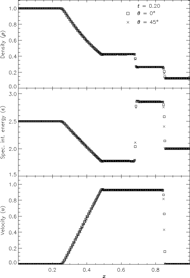
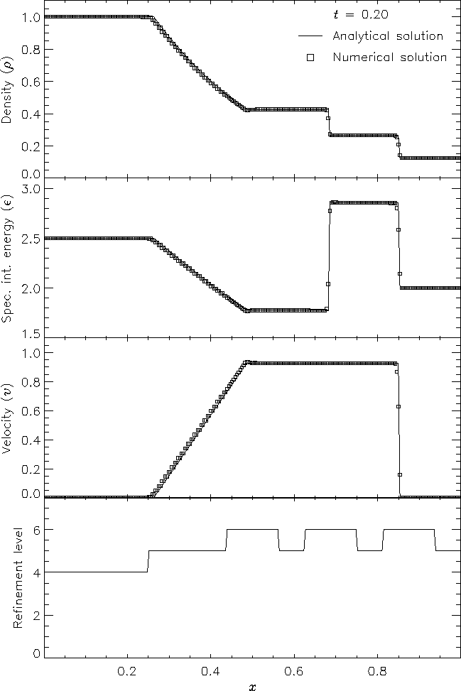
Figure 6 shows the result of running the Sod problem with FLASH on a two-dimensional grid, with the analytical solution shown for comparison. The hydrodynamical algorithm used here is the directionally split piecewise-parabolic method (PPM) included with FLASH. In this run the shock normal is chosen to be parallel to the x-axis. With six levels of refinement, the effective grid size at the finest level is 2562, so the finest zones have width 0.00390625. At t = 0.2 three different nonlinear waves are present: a rarefaction between x » 0.25 and x » 0.5, a contact discontinuity at x » 0.68, and a shock at x » 0.85. The two sharp discontinuities are each resolved with approximately three zones at the highest level of refinement, demonstrating the ability of PPM to handle sharp flow features well. Near the contact discontinuity and in the rarefaction we find small errors of about 1-2% in the density and specific internal energy, with similar errors in the velocity inside the rarefaction. Elsewhere the numerical solution is exact; no oscillation is present.
Figure 7 shows the result of running the Sod problem on the same two-dimensional grid with different shock normals: parallel to the x-axis (q = 0°) and along the box diagonal (q = 45°). For the diagonal solution we have interpolated values of density, specific internal energy, and velocity to a set of 256 points spaced exactly as in the x-axis solution. This comparison shows the effects of the second-order directional splitting used with FLASH on the resolution of shocks. At the right side of the rarefaction and at the contact discontinuity the diagonal solution undergoes slightly larger oscillations (on the order of a few percent) than the x-axis solution. Also, the value of each variable inside the discontinuity regions differs between the two solutions by up to 10% in most cases. However, the location and thickness of the discontinuities is the same between the two solutions. In general shocks at an angle to the grid are resolved with approximately the same number of zones as shocks parallel to a coordinate axis.

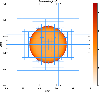
Figure 8 presents a grayscale map of the density at t = 0.2 in the diagonal solution together with the block structure of the AMR grid in this case. Note that regions surrounding the discontinuities are maximally refined, while behind the shock and discontinuity the grid has de-refined as the second derivative of the density has decreased in magnitude. Because zero-gradient outflow boundaries were used for this test, some reflections are present at the upper left and lower right corners, but at t = 0.2 these have not yet propagated to the center of the grid.
This problem was originally used by Woodward and Colella (1984) to compare the performance of several different hydrodynamical methods on problems involving strong, thin shock structures. It has no analytical solution, but since it is one-dimensional, it is easy to produce a converged solution by running the code with a very large number of zones, permitting an estimate of the self-convergence rate when narrow, interacting discontinuities are present. For FLASH it also provides a good test of the adaptive mesh refinement scheme.
The initial conditions consist of two parallel, planar flow discontinuities. Reflecting boundary conditions are used. The density in the left, middle, and right portions of the grid (rL, rM, and rR, respectively) is unity; everywhere the velocity is zero. The pressure is large to the left and right and small in the center:
| (38) |
Figure 9 shows the density and velocity profiles at several different times in the converged solution, demonstrating the complexity inherent in this problem. The initial pressure discontinuities drive shocks into the middle part of the grid; behind them, rarefactions form and propagate toward the outer boundaries, where they are reflected back onto the grid and interact with themselves. By the time the shocks collide at t = 0.028, the reflected rarefactions have caught up to them, weakening them and making their post-shock structure more complex. Because the right-hand shock is initially weaker, the rarefaction on that side reflects from the wall later, so the resulting shock structures going into the collision from the left and right are quite different. Behind each shock is a contact discontinuity left over from the initial conditions (at x » 0.50 and 0.73). The shock collision produces an extremely high and narrow density peak; in the Woodward and Colella calculation the peak density is slightly less than 30. Even with ten levels of refinement, FLASH obtains a value of only 18 for this peak. Reflected shocks travel back into the colliding material, leaving a complex series of contact discontinuities and rarefactions between them. A new contact discontinuity has formed at the point of the collision (x » 0.69). By t = 0.032 the right-hand reflected shock has met the original right-hand contact discontinuity, producing a strong rarefaction which meets the central contact discontinuity at t = 0.034. Between t = 0.034 and t = 0.038 the slope of the density behind the left-hand shock changes as the shock moves into a region of constant entropy near the left-hand contact discontinuity.
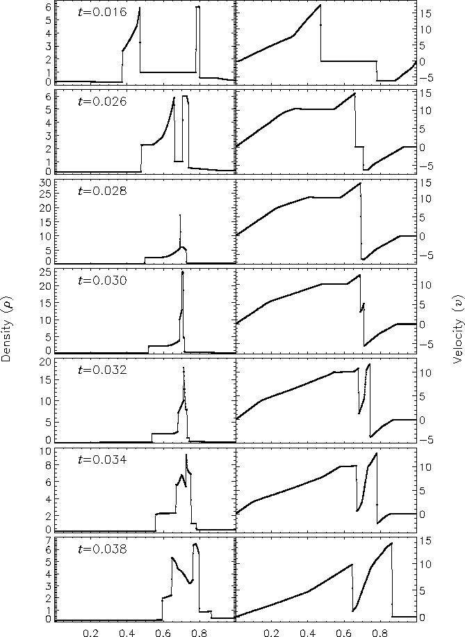
Figure 10 shows the self-convergence of density and pressure when FLASH is run on this problem. For several runs with different maximum refinement levels, we compare the density, pressure, and total specific energy at t = 0.038 to the solution obtained using FLASH with ten levels of refinement. This figure plots the L1 error norm for each variable u, defined using
| (39) |
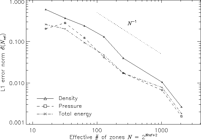
Although PPM is formally a second-order method, one sees from this plot that, for the interacting blast-wave problem, the convergence rate is only linear. Indeed, in their comparison of the performance of seven nominally second-order hydrodynamic methods on this problem, Woodward and Colella found that only PPM achieved even linear convergence; the other methods were worse. The error norm is very sensitive to the correct position and shape of the strong, narrow shocks generated in this problem.
The additional runtime parameters supplied with the 2blast problem are listed in Table 2. This problem is configured to use the perfect-gas equation of state (eos/gamma), and it is run in a two-dimensional unit box with gamma set to 1.4. Boundary conditions in the y direction (transverse to the shock normals) are taken to be periodic.
| Variable | Type | Default | Description |
| rho_left | real | 1 | Initial density to the left of the left interface (rL) |
| rho_mid | real | 1 | Initial density between the interfaces (rM) |
| rho_right | real | 1 | Initial density to the right of the right interface (rR) |
| p_left | real | 1000 | Initial pressure to the left (pL) |
| p_mid | real | 0.01 | Initial pressure in the middle (pM) |
| p_right | real | 100 | Initial pressure to the right (pR) |
| u_left | real | 0 | Initial velocity (perpendicular to interface) to the left (uL) |
| u_mid | real | 0 | Initial velocity (perpendicular to interface) in the middle (uL) |
| u_right | real | 0 | Initial velocity (perpendicular to interface) to the right (uR) |
| xangle | real | 0 | Angle made by interface normal with the x-axis (degrees) |
| yangle | real | 90 | Angle made by interface normal with the y-axis (degrees) |
| posnL | real | 0.1 | Point of intersection between the left interface plane and the x-axis |
| posnR | real | 0.9 | Point of intersection between the right interface plane and the x-axis |
The Sedov explosion problem (Sedov 1959) is another purely hydrodynamical test in which we check the code's ability to deal with strong shocks and non-planar symmetry. The problem involves the self-similar evolution of a cylindrical or spherical blast wave from a delta-function initial pressure perturbation in an otherwise homogeneous medium. To initialize the code, we deposit a quantity of energy E = 1 into a small region of radius dr at the center of the grid. The pressure inside this volume, p0˘, is given by
| (40) |
| (41) |
| |||||||||||||||||||||||||
| |||||||||||||||||||
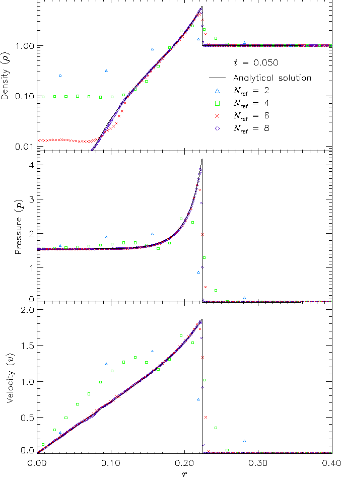
Figure 11 shows density, pressure, and velocity profiles in the two-dimensional Sedov problem at t = 0.05. Solutions obtained with FLASH on grids with 2, 4, 6, and 8 levels of refinement are shown in comparison with the analytical solution. In this figure we have computed average radial profiles in the following way. We interpolated solution values from the adaptively gridded mesh used by FLASH onto a uniform mesh having the same resolution as the finest AMR blocks in each run. Then, using radial bins with the same width as the zones in the uniform mesh, we binned the interpolated solution values, computing the average value in each bin. At low resolutions, errors show up as density and velocity overestimates behind the shock, underestimates of each variable within the shock, and a numerical precursor spanning 1-2 zones in front of the shock. However, the central pressure is accurately determined, even for two levels of refinement; because the density goes to a finite value rather than its correct limit of zero, this corresponds to a finite truncation of the temperature (which should go to infinity as r® 0). As resolution improves, the artificial finite density limit decreases; by Nref = 6 it is less than 0.2% of the peak density. Except for the Nref = 2 case, which does not show a well-defined peak in any variable, the shock itself is always captured with about two zones. The region behind the shock containing 90% of the swept-up material is represented by four zones in the Nref = 4 case, 17 zones in the Nref = 6 case, and 69 zones for Nref = 8. However, because the solution is self-similar, for any given maximum refinement level the shock will be four zones wide at a sufficiently early time. The behavior when the shock is underresolved is to underestimate the peak value of each variable, particularly the density and pressure.
Figure 12 shows the pressure field in the 8-level calculation at t = 0.05 together with the block refinement pattern. Note that a relatively small fraction of the grid is maximally refined in this problem. Although the pressure gradient at the center of the grid is small, this region is refined because of the large temperature gradient there. This illustrates the ability of PARAMESH to refine grids using several different variables at once.
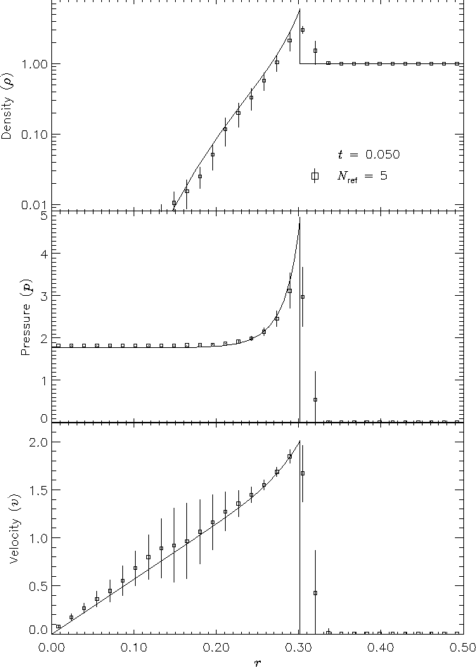
We have also run FLASH on the spherically symmetric Sedov problem in order to verify the code's performance in three dimensions. The results at t = 0.05 using five levels of grid refinement are shown in Figure 13. In this figure we have plotted the root-mean-square (RMS) numerical solution values in addition to the average values. As in the two-dimensional runs, the shock is spread over about two zones at the finest AMR resolution in this run. The width of the pressure peak in the analytical solution is about 1 1/2 zones at this time, so the maximum pressure is not captured in the numerical solution. Behind the shock the numerical solution average tracks the analytical solution quite well, although the Cartesian grid geometry produces RMS deviations of up to 40% in the density and velocity in the derefined region well behind the shock. This behavior is similar to that exhibited in the two-dimensional problem at comparable resolution.
| Variable | Type | Default | Description |
| p_ambient | real | 10-5 | Initial ambient pressure (p0) |
| rho_ambient | real | 1 | Initial ambient density (r0) |
| exp_energy | real | 1 | Explosion energy (E) |
| r_init | real | 0.05 | Radius of initial pressure perturbation (dr) |
| xctr | real | 0.5 | x-coordinate of explosion center |
| yctr | real | 0.5 | y-coordinate of explosion center |
| zctr | real | 0.5 | z-coordinate of explosion center |
The additional runtime parameters supplied with the sedov problem are listed in Table 3. This problem is configured to use the perfect-gas equation of state (eos/gamma), and it is run in a unit box with gamma set to 1.4.
In this problem we create a planar density pulse in a region of uniform pressure p0 and velocity u0, with the velocity normal to the pulse plane. The density pulse is defined via
| (44) |
| (45) |
| (46) |
The advection problem tests the ability of the code to handle planar geometry, as does the Sod problem. It is also like the Sod problem in that it tests the code's treatment of flow discontinuities which move at one of the characteristic speeds of the hydrodynamical equations. (This is difficult because noise generated at a sharp interface, such as the contact discontinuity in the Sod problem, tends to move with the interface, accumulating there as the calculation advances.) However, unlike the Sod problem it compares the code's treatment of leading and trailing contact discontinuities (for the square pulse), and it tests the treatment of narrow flow features (for both the square and Gaussian pulse shapes). Many hydrodynamical methods have a tendency to clip narrow features or to distort pulse shapes by introducing artificial dispersion and dissipation (Zalesak 1987).
| Variable | Type | Default | Description |
| rhoin | real | 1 | Characteristic density inside the advected pulse (r1) |
| rhoout | real | 10-5 | Ambient density (r0) |
| pressure | real | 1 | Ambient pressure (p0) |
| velocity | real | 10 | Ambient velocity (u0) |
| width | real | 0.1 | Characteristic width of advected pulse (w) |
| pulse_fctn | integer | 1 | Pulse shape function to use: 1=square wave, 2=Gaussian |
| xangle | real | 0 | Angle made by pulse plane with x-axis (degrees) |
| yangle | real | 90 | Angle made by pulse plane with y-axis (degrees) |
| posn | real | 0.25 | Point of intersection between pulse midplane and x-axis |
The additional runtime parameters supplied with the advect problem are listed in Table 4. This problem is configured to use the perfect-gas equation of state (eos/gamma), and it is run in a unit box with gamma set to 1.4. (The value of g does not affect the analytical solution, but it does affect the timestep.)
To demonstrate the performance of FLASH on the advection problem, we have performed tests of both the square and Gaussian pulse profiles with the pulse normal parallel to the x-axis (q = 0°) and at an angle to the x-axis (q = 45°) in two dimensions. The square pulse used r1 = 1, r0 = 10-3, p0 = 10-6, u0 = 1, and w = 0.1. With six levels of refinement in the domain [0,1]×[0,1], this value of w corresponds to having about 52 zones across the pulse width. The Gaussian pulse tests used the same values of r1, r0, p0, and u0, but with w = 0.015625. This value of w corresponds to about 8 zones across the pulse width at six levels of refinement. For each test we performed runs at two, four, and six levels of refinement to examine the quality of the numerical solution as the resolution of the advected pulse improves. The runs with q = 0° used zero-gradient (outflow) boundary conditions, while the runs performed at an angle to the x-axis used periodic boundaries.
Figure 14 shows, for each test, the advected density profile at t = 0.4 in comparison with the analytical solution. The upper two frames of this figure depict the square pulse with q = 0° and q = 45°, while the lower two frames depict the Gaussian pulse results. In each case the analytical density pulse has been advected a distance u0t = 0.4, and in the figure the axis parallel to the pulse normal has been translated by this amount, permitting comparison of the pulse displacement in the numerical solutions with that of the analytical solution.
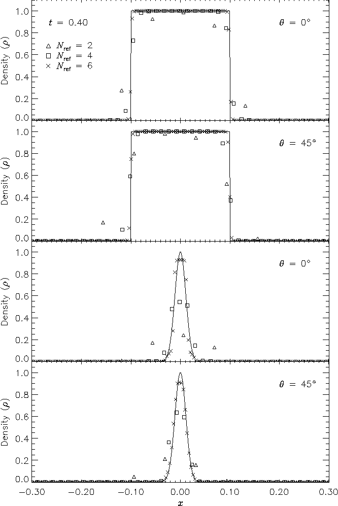
The advection results show the expected improvement with increasing AMR refinement level Nref. Inaccuracies appear as diffusive spreading, rounding of sharp corners, and clipping. In both the square pulse and Gaussian pulse tests, diffusive spreading is limited to about one zone on either side of the pulse. For Nref = 2 the rounding of the square pulse and the clipping of the Gaussian pulse are quite severe; in the latter case the pulse itself spans about two zones, which is the approximate smoothing length in PPM for a single discontinuity. For Nref = 4 the treatment of the square pulse is significantly better, but the amplitude of the Gaussian is still reduced by about 50%. In this case the square pulse discontinuities are still being resolved with 2-3 zones, but the zones are now a factor of 25 smaller than the pulse width. With six levels of refinement the same behavior is observed for the square pulse, while the amplitude of the Gaussian pulse is now 93% of its initial value. The absence of dispersive effects (ie. oscillation) despite the high order of the PPM interpolants is due to the enforcement of monotonicity in the PPM algorithm.
The diagonal runs are consistent with the runs which were parallel to the x-axis, with the possibility of a slight amount of extra spreading behind the pulse. However, note that we have determined density values for the diagonal runs by interpolation along the grid diagonal. The interpolation points are not centered on the pulses, so the density does not always take on its maximum value (particularly in the lowest-resolution case).
These results are consistent with earlier studies of linear advection with PPM (e.g., Zalesak 1987). They suggest that, in order to preserve narrow flow features in FLASH, the maximum AMR refinement level should be chosen so that zones in refined regions are at least a factor 5-10 smaller than the narrowest features of interest. In cases in which the features are generated by shocks (rather than moving with the fluid), the resolution requirement is not as severe, as errors generated in the preshock region are driven into the shock rather than accumulating as it propagates.
The problem of a wind tunnel containing a step was first described by Emery (1968), who used it to compare several hydrodynamical methods which are only of historical interest now. Woodward and Colella (1984) later used it to compare several more advanced methods, including PPM. Although it has no analytical solution, this problem is useful because it exercises a code's ability to handle unsteady shock interactions in multiple dimensions. It also provides an example of the use of FLASH to solve problems with irregular boundaries.
The problem uses a two-dimensional rectangular domain three units wide and one unit high. Between x = 0.6 and x = 3 along the x-axis is a step 0.2 units high. The step is treated as a reflecting boundary, as are the lower and upper boundaries in the y direction. For the right-hand x boundary we use an outflow (zero gradient) boundary condition, while on the left-hand side we use an inflow boundary. In the inflow boundary zones we set the density to r0, the pressure to p0, and the velocity to u0, with the latter directed parallel to the x-axis. The domain itself is also initialized with these values. For the Emery problem we use
| (47) |
The additional runtime parameters supplied with the windtunnel problem are listed in Table 5. This problem is configured to use the perfect-gas equation of state (eos/gamma) with gamma set to 1.4. We also set xmax = 3, ymax = 1, Nblockx = 15, and Nblocky = 4 in order to create a grid with the correct dimensions. The version of divide_domain supplied with this problem adds three top-level blocks along the lower left-hand corner of the grid to cover the region in front of the step. Finally, we use xlboundary = -23 (user boundary condition) and xrboundary = -21 (outflow boundary) to instruct FLASH to use the correct boundary conditions in the x direction. Boundaries in the y direction are reflecting (-20).
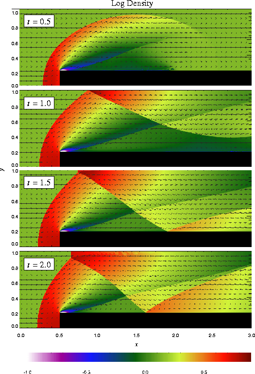
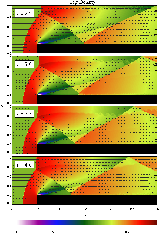
Until t = 12 the flow is unsteady, exhibiting multiple shock reflections and interactions between different types of discontinuity. Figure 15 shows the evolution of density and velocity between t = 0 and t = 4 (the period considered by Woodward and Colella). Immediately a shock forms directly in front of the step and begins to move slowly away from it. Simultaneously the shock curves around the corner of the step, extending farther downstream and growing in size until it strikes the upper boundary just after t = 0.5. The corner of the step becomes a singular point, with a rarefaction fan connecting the still gas just above the step to the shocked gas in front of it. Entropy errors generated in the vicinity of this singular point produce a numerical boundary layer about one zone thick along the surface of the step. Woodward and Colella reduce this effect by resetting the zones immediately behind the corner to conserve entropy and the sum of enthalpy and specific kinetic energy through the rarefaction. However, we are less interested here in reproducing the exact solution than in verifying the code and examining the behavior of such numerical effects as resolution is increased, so we do not apply this additional boundary condition. The errors near the corner result in a slight overexpansion of the gas there and a weak oblique shock where this gas flows back toward the step. At all resolutions we also see interactions between the numerical boundary layer and the reflected shocks which appear later in the calculation.
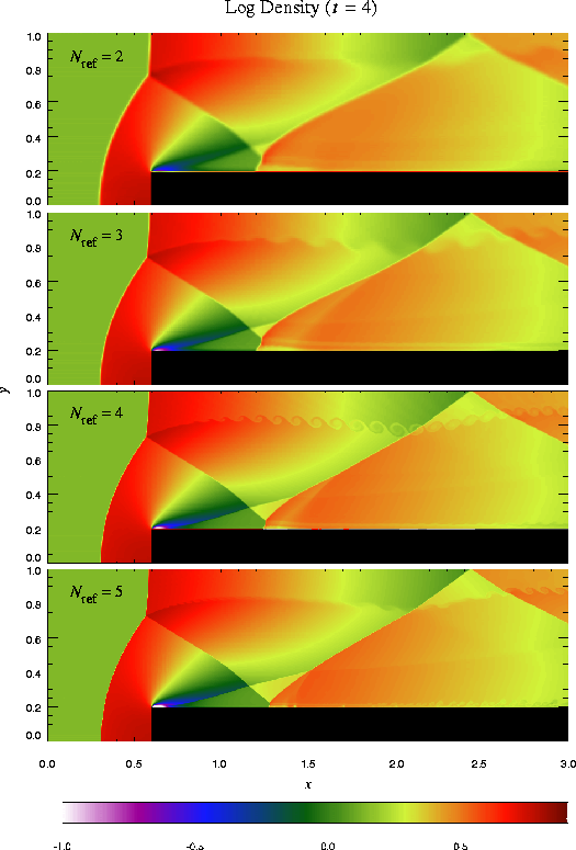
By t = 1 the shock reflected from the upper wall has moved downward and has almost struck the top of the step. The intersection between the primary and reflected shocks begins at x » 1.45 when the reflection first forms at t » 0.65, then moves to the left, reaching x » 0.95 at t = 1. As it moves, the angle between the incident shock and the wall increases until t = 1.5, at which point it exceeds the maximum angle for regular reflection (40° for g = 1.4) and begins to form a Mach stem. Meanwhile the reflected shock has itself reflected from the top of the step, and here too the point of intersection moves leftward, reaching x » 1.65 by t = 2. The second reflection propagates back toward the top of the grid, reaching it at t = 2.5 and forming a third reflection. By this time in low-resolution runs we see a second Mach stem forming at the shock reflection from the top of the step; this results from the interaction of the shock with the numerical boundary layer, which causes the angle of incidence to increase faster than in the converged solution. Figure 16 compares the density field at t = 4 as computed by FLASH using several different maximum levels of refinement. Note that the size of the artificial Mach reflection diminishes as resolution improves.
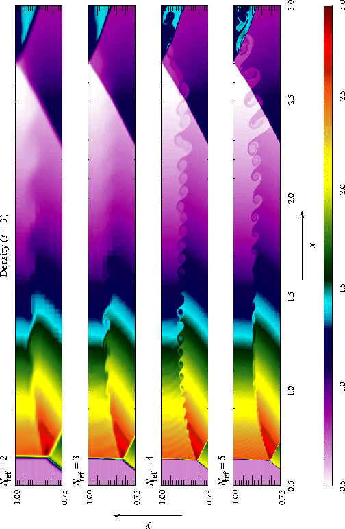
The shear zone behind the first (``real'') Mach stem produces another interesting numerical effect, visible at t = 3 and t = 4: Kelvin-Helmholtz amplification of numerical errors generated at the shock intersection. The wave thus generated propagates downstream and is refracted by the second and third reflected shocks. This effect is also seen in the calculations of Woodward and Colella, although their resolution was too low to capture the detailed eddy structure we see. Figure 17 shows the detail of this structure at t = 3 on grids with several different levels of refinement. The effect does not disappear with increasing resolution, for two reasons. First, the instability amplifies numerical errors generated at the shock intersection, no matter how small. Second, PPM captures the slowly moving, nearly vertical Mach stem with only 1-2 zones on any grid, so as it moves from one column of zones to the next, artificial kinks form near the intersection, providing the seed perturbation for the instability. This effect can be reduced by using a small amount of extra dissipation to smear out the shock, as discussed by Colella and Woodward (1984). This tendency of physical instabilities to amplify numerical noise vividly demonstrates the need to exercise caution when interpreting features in supposedly converged calculations.
Finally, we note that in high-resolution runs with FLASH we also see some Kelvin-Helmholtz rollup at the numerical boundary layer along the top of the step. This is not present in Woodward and Colella's calculation, presumably because their grid resolution is lower (corresponding to two levels of refinement for us) and because of their special treatment of the singular point.
| Variable | Type | Default | Description |
| p_ambient | real | 1 | Ambient pressure (p0) |
| rho_ambient | real | 1.4 | Ambient density (r0) |
| wind_vel | real | 3 | Inflow velocity (u0) |
![]() Go on to Section 6.
Go on to Section 6.