22.3 Unit Test

FLASH provides a unit test for checking the basic functionality of the Cosmology module. It tests the unit's generated cosmological scaling factor, cosmological redshift, and the time calculated from that redshift against an analytical solution of these quantities.

The test is run with the following parameters:

OmegaMatter = 1.0
OmegaLambda = 0.0
OmegaBaryon = 1.0
OmegaRadiation = 0.0
HubbleConstant = $1.62038\times10^{-18} {\rm sec}^{-1}$ (50 km/s/Mpc)

The Cosmological scaling factor is related to time by the equation:

$a(t)={\left(\frac{t}{t_0}\right)}^{2/3}$

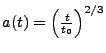
where $t_0=\frac{2}{3H_0}$, $H_0$ is the HubbleConstant and is related to the cosmological redshift by the equation $z(t)=\frac{1}{a(t)}-1$. The change in time is a uniform step, and by comparing the analytical and code results at time $t$, we can see if the Friedmann equations are correctly integrated by the Cosmology unit, and that the results fall within a tolerance set in Cosmology_unitTest.