32.2 Piecewise Cubic Interpolation
Piecewise cubic interpolation is a technique that can be used to create functional  surfaces
(1st derivative continuous) throughout a grid domain by using functional and derivative information at
each vertex of a grid cell. The domain function
surfaces
(1st derivative continuous) throughout a grid domain by using functional and derivative information at
each vertex of a grid cell. The domain function  and its derivatives
  are assumed
to be known or at least calculable at each vertex. In order to show the essential features of the
piecewise cubic interpolation method and to keep the formulas and matrix sizes manageable, we present the
method for 2D domain geometries.
are assumed
to be known or at least calculable at each vertex. In order to show the essential features of the
piecewise cubic interpolation method and to keep the formulas and matrix sizes manageable, we present the
method for 2D domain geometries.
Consider a particular rectangular 2D cell. We wish to calculate a domain function as a
piecewise cubic polynomial in terms of ![$ [0,1]$](img1397.png) rescaled variables
rescaled variables  inside each cell:
The rescaled variable  is obtained from the domain global variable
  and the cell's
lower
and the cell's
lower  and upper
  dimension as
with a similar expression for  . From the expansion in 32.1, there are 16 expansion
coefficients which need to be determined (fitted) to an appropriate set of data for specific points
on the cell, which, in order to assure continuous representation of over the entire domain, have
to sit on the cell's boundaries. The most obvious choice for these points are the cell vertices, each
vertex belonging to four cells. The data needed for each vertex are ,
. From the expansion in 32.1, there are 16 expansion
coefficients which need to be determined (fitted) to an appropriate set of data for specific points
on the cell, which, in order to assure continuous representation of over the entire domain, have
to sit on the cell's boundaries. The most obvious choice for these points are the cell vertices, each
vertex belonging to four cells. The data needed for each vertex are ,  ,
,  and
and  .
This leads to a linearly independent and rotationally invariant set of 16 data values, from which the
16 expansion coefficients can be uniquely determined. It can also be shown that for other dimensions
only the inclusion of all mixed simple higher order derivatives leads to a linearly independent
and rotationally invariant set of data values. For example, for rectangular 3D geometries the data needed at
each of the 8 vertices of a cubic cell is , , ,
.
This leads to a linearly independent and rotationally invariant set of 16 data values, from which the
16 expansion coefficients can be uniquely determined. It can also be shown that for other dimensions
only the inclusion of all mixed simple higher order derivatives leads to a linearly independent
and rotationally invariant set of data values. For example, for rectangular 3D geometries the data needed at
each of the 8 vertices of a cubic cell is , , ,  , ,
, ,  ,
,
 and
and
 .
.
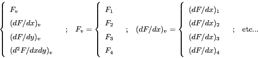
Let us now organize the 16 expansion coefficients  into a vector
  , such that each
element
, such that each
element  of is associated with the following expansion coefficient:
Likewise, we stack the data values of the four vertices  into a vector
  as follows:
Let us associate the four vertex indices with the following four rescaled variables of the cell:
| |
|
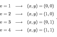 |
(32.5) |
Substituting these values for and into equation 32.1 and its derivatives, we can
establish a connection between the expansion coefficient vector and the data vector in the form
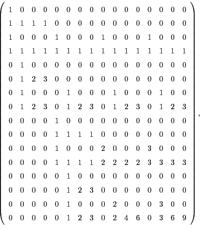
where the 16 x 16 matrix  has the following structure
containing only positive integers and many zeros (175 out of 256 elements). Since we are ultimately
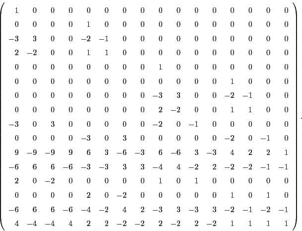
interested in the expansion coefficients for the cell, we invert equation 32.6 and get
The inverse
 is also an integer matrix and again contains many zero elements,
although not as many as itself (156 out of 256 elements):
is also an integer matrix and again contains many zero elements,
although not as many as itself (156 out of 256 elements):
The matrix
is universal for all 2D cells. Each cell has
its specific data vector from which its expansion coefficient vector can be established
via 32.8. Rather than storing
in matrix form and performing a direct matrix
times vector operation for each cell,
is used implicitly when converting
to . This avoids the redundant zero multiplications and is thus much more efficient.
In fact, by using cleverly arranged reusable intermediates, this to transformation can
be coded using only additions and subtractions and no multiplications at all.
Once the expansion coefficient vector for a cell has been established, equation 32.1
can be used to obtain the function value at any point inside the cell, provided the rescaled
coordinates of that point are given. The function values are given by Eq.(32.1), which can be
computed efficiently using a double Horner scheme:
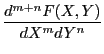
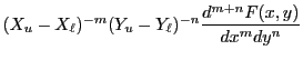
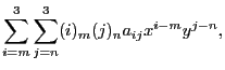
The evaluation of the global coordinate differentials is done using the chain rule and leads to:
where the Pochhammer symbol  is defined as
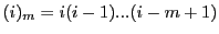 .
.