27.2 Profiler

Figure 27.2: The Profiler unit directory tree.

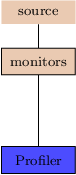
In addition to an interface for simple timers, FLASH includes a generic interface for third-party profiling or tracing libraries. This interface is defined in the monitors/Profiler unit.

In FLASH4 we created an interface to the IBM profiling libraries libmpihpm.a and libmpihpm_smp.a and also to HPCToolkit http://hpctoolkit.org/ (Rice University). We make use of this interface to profile FLASH evolution only, i.e. not initialization. To use this style of profiling add -unit=monitors/Profiler/ProfilerMain/mpihpm or -unit=monitors/Profiler/ProfilerMain/hpctoolkit to your setup line and also set the FLASH runtime parameter profileEvolutionOnly = .true.

For the IBM profiling library (mpihpm) you need to add LIB_MPIHPM and LIB_MPIHPM_SMP macros to your Makefile.h to link FLASH to the profiling libraries. The actual macro used in the link line depends on whether you setup FLASH with multithreading support (LIB_MPIHPM for MPI-only FLASH and LIB_MPIHPM_SMP for multithreaded FLASH). Example values from sites/miralac1/Makefile.h follow

 

LIB_MPI =
HPM_COUNTERS = /bgsys/drivers/ppcfloor/bgpm/lib/libbgpm.a
LIB_MPIHPM = -L/soft/perftools/hpctw -lmpihpm 
$(HPM_COUNTERS)$(LIB_MPI)
LIB_MPIHPM_SMP = -L/soft/perftools/hpctw -lmpihpm_smp 
$(HPM_COUNTERS)$(LIB_MPI)

For HPCToolkit you need to set the environmental variable HPCRUN_DELAY_SAMPLING=1 at job launch to enable selective profiling (see the HPCToolkit user guide).