Next: 27.2 Profiler Up: 27. Timer and Profiler Previous: 27. Timer and Profiler Contents Index
The performance routines start or stop a timer at the beginning or end of a section of code to be monitored, and accumulate performance information in dynamically assigned accounting segments. The code also has an interface to write the timing summary to the FLASH logfile. These routines are not recommended for timing very short segments of code due to the overhead in accounting.
There are two ways of using the Timers routines in your code. One mode is to simply pass timer names as strings to the start and stop routines. In this first way, a timer with the given name will be created if it doesn't exist, or otherwise reference the one already in existence. The second mode of using the timers references them not by name but by an integer key. This technique offers potentially faster access if a timer is to be started and stopped many times (although still not recommended because of the overhead). The integer key is obtained by calling with a string name Timers_create which will only create the timer if it doesn't exist and will return the integer key. This key can then be passed to the start and stop routines.
The typical usage pattern for the timers is implemented in the default Driver implementation. This pattern is: call Timers_init once at the beginning of a run, call Timers_start and Timers_stop around sections of code, and call Timers_getSummary at the end of the run to report the timing summary at the end of the logfile. However, it is possible to call Timers_reset in the middle of a run to reset all timing information. This could be done along with writing the summary once per-timestep to report code times on a per-timestep basis, which might be relevant, for instance, for certain non-fixed operation count solvers. Since Timers_reset does not reset the integer key mappings, it is safe to obtain a key through Timers_create once in a saved variable, and continue to use it after calling Timers_reset.
Two runtime parameters control the Timer unit and are described below.
| Parameter | Type | Default value | Description |
| eachProcWritesSummary | LOGICAL | TRUE | Should each process write
its summary to its own file? If true, each
process will write its summary to a file named timer_summary_ |
| writeStatSummary | LOGICAL | TRUE | Should timers write the max/min/avg values for timers to the logfile? |
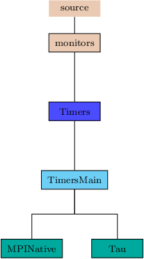
monitors/Timers/TimersMain/MPINative writes two summaries to the logfile:
the first gives the timer execution of the master
processor, and the second gives the statistics of max, min, and avg
times for timers on all processors. The secondary max, min, and avg times will not be
written if some process executed timers differently than another. For example,
this anomaly happens if not all processors contain at least one block. In this case,
the Hydro timers only execute on the processors that possess blocks.
See Sec:LogfilePerformance for an example of this type of output.
The max, min, and avg summary can be disabled by setting the runtime parameter
writeStatSummary to false. In addition, each process can write its
summary to its own file named timer_summary_![]() process id
process id![]() . To prohibit
each process from writing its summary to its own file, set the runtime
parameter eachProcWritesSummary to false.
. To prohibit
each process from writing its summary to its own file, set the runtime
parameter eachProcWritesSummary to false.
To use this implementation we must compile the FLASH source code with the Tau compiler wrapper scripts. These are set as the default compilers automatically whenever we specify the -tau option (see Sec:ListSetupArgs) to the setup script. In addition to the -tau option we must specify -with-unit=monitors/Timers/TimersMain/Tau as this Timers implementation is not the default.