8.1 Overview

The Grid unit has four subunits: GridMain is responsible for maintaining the Eulerian grid used to discretize the spatial dimensions of a simulation; GridParticles manages the data movement related to active, and Lagrangian tracer particles; GridBoundaryConditions handles the application of boundary conditions at the physical boundaries of the domain; and GridSolvers provides services for solving some types of partial differential equations on the grid. 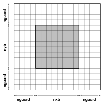In the Eulerian grid, discretization is achieved by dividing the computational domain into one or more sub-domains or blocks, and using these blocks as the primary computational entity visible to the physics units. A block contains a number of computational cells (nxb in the $x$-direction, nyb in the $y$-direction, and nzb in the $z$-direction). A perimeter of guardcells, of width nguard cells in each coordinate direction, surrounds each block of local data, providing it with data from the neighboring blocks or with boundary conditions, as shown in Figure 8.4. Since the majority of physics solvers used in FLASH are explicit, a block with its surrounding guard cells becomes a self-contained computational domain. Thus the physics units see and operate on only one block at a time, and this abstraction is reflected in their design.

Therefore any mesh package that can present a self contained block as a computational domain to a client unit can be used with FLASH. However, such interchangeability of grid packages also requires a careful design of the Grid API to make the underlying management of the discretized grid completely transparent to outside units. The data structures for physical variables, the spatial coordinates, and the management of the grid are kept private to the Grid unit, and client units can access them only through accessor functions. This strict protocol for data management along with the use of blocks as computational entities enables FLASH to abstract the grid from physics solvers and facilitates the ability of FLASH to use multiple mesh packages.

Figure 8.4: A single 2-D block showing the interior cells (shaded) and the perimeter of guard cells.

Any unit in the code can retrieve all or part of a block of data from the Grid unit along with the coordinates of corresponding cells; it can then use this information for internal computations, and finally return the modified data to the Grid unit. The Grid unit also manages the parallelization of FLASH. It consists of a suite of subroutines which handle distribution of work to processors and guard cell filling. When using an adaptive mesh, the Grid unit is also responsible for refinement/derefinement and conservation of flux across block boundaries.

FLASH can interchangeably use either a uniform or adaptive grid for most problems. Additionally, a new feature in FLASH4 is an option to replicate the mesh; that is processors are assumed to be partitioned into groups, each group gets a copy of the entire domain mesh. This feature is useful when it is possible to decompose the computation based upon certain compute intensive tasks that apply across the domain. One such example is radiation transfer with multigroup flux limited diffusion where each group needs an implicit solve. Here the state variable of the mesh are replicated on each group of processors, while the groups are unique. Thus at the cost of some memory redundancy, it becomes possible to compute a higher fidelity problem (see chp:RadTrans for an example). Because of this feature, the parallel environment of the simulation is now controlled by the Driver which differentiates between global communicators and mesh communicators. The Grid unit queries the Driver unit for mesh communicators. In all other respects this change is transparent to the Grid unit. Mesh replication can be invoked through the runtime parameter meshCopyCount

The uniform grid supported in FLASH discretizes the physical domain by placing grid points at regular intervals defined by the geometry of the problem. The grid configuration remains unchanged throughout the simulation, and exactly one block is mapped per processor. An adaptive grid changes the discretization over the course of the computation, and several blocks can be mapped to each computational processor. Two AMR packages are currently supported in FLASH for providing adaptive grid capbility. The block-structured oct-tree based AMR package, PARAMESH has been the work horse since the beginning of the code. Version 2 and Version 4 of paramesh are both supported, version 2 is kept mostly to enable cross checking against FLASH2 results. FLASH4, for the first time, includes patch based Chombo as an alternative AMR package. By default, PARAMESH 4 is chosen when setting up an application, unless another implementation is explicitly specified. The use of paramesh 2 is deprecated, and Chombo has not so far been used for production at the Flash Center.

FLASH3 Transition: The following two commands will create the same (identical) application: a simulation of a Sod shock tube in 3 dimensions with PARAMESH 4 managing the grid.  

./setup Sod -3d -auto


./setup Sod -3d -auto -unit=Grid/GridMain/paramesh/paramesh4/Paramesh4.0

However, if the command is changed to  

./setup Sod -3d -auto -unit=Grid/GridMain/UG

the application is set up with a uniform grid instead. Additionally, because two different grids types are supported in FLASH, the user must match up the correct IO alternative implementation with the correct Grid alternative implementation. Please see Chp:IO for more details. Note that the setup script has capabilities to let the user set up shortcuts, such as “+ugio”, which makes sure that the appropriate branch of IO is included when the uniform grid is being used. Please see Sec:SetupShortcuts for more information. Also see grid tips for shortcuts useful for the Grid unit.