Next:
17.1 Introduction
Up:
V. Physics Units
Previous:
16. Incompressible Navier-Stokes Unit
Contents
Index
17
. Equation of State Unit
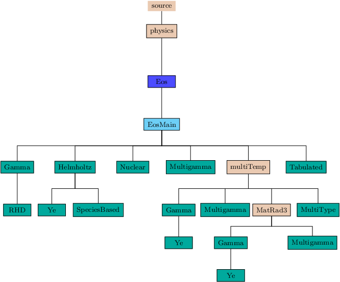
Figure 17.1:
The
Eos
directory tree.
Subsections
17
.
1
Introduction
17
.
2
Gamma Law and Multigamma
17
.
2
.
1
Ideal Gamma Law for Relativistic Hydrodynamics
17
.
3
Helmholtz
17
.
4
Multitemperature extension for Eos
17
.
4
.
1
Gamma
17
.
4
.
1
.
1
Gamma/Ye
17
.
4
.
2
Multigamma
17
.
4
.
3
Tabulated
17
.
4
.
3
.
1
SESAME TEOS
17
.
4
.
3
.
2
Interpolation strategy for SESAME
17
.
4
.
3
.
3
Use of the SESAME database
17
.
4
.
3
.
4
Types and structures thereof of SESAME data records
17
.
4
.
3
.
5
Example format of a SESAME table
17
.
4
.
4
Multitype
17
.
5
MultiFluid
17
.
6
Usage
17
.
6
.
1
Initialization
17
.
6
.
2
Runtime Parameters
17
.
6
.
3
Direct and Wrapped Calls
17
.
7
Unit Test