2.4 Running FLASH

We are now ready to run FLASH. To run FLASH on N processors, type

mpirun -np N flashX

remembering to replace N and X with the appropriate values. Some systems may require you to start MPI programs with a different command; use whichever command is appropriate for your system. The FLASH4 executable accepts an optional command-line argument for the runtime parameters file. If “-par_file filename” is present, FLASH reads the file specified on command line for runtime parameters, otherwise it reads flash.par.

You should see a number of lines of output indicating that FLASH is initializing the Sedov problem, listing the initial parameters, and giving the timestep chosen at each step. After the run is finished, you should find several files in the current directory:

• sedov.log echoes the runtime parameter settings and indicates the run time, the build time, and the build machine. During the run, a line is written for each timestep, along with any warning messages. If the run terminates normally, a performance summary is written to this file.
• sedov.dat contains a number of integral quantities as functions of time: total mass, total energy, total momentum, etc. This file can be used directly by plotting programs such as gnuplot; note that the first line begins with a hash (#) and is thus ignored by gnuplot.

• sedov_hdf5_chk_000* are the different checkpoint files. These are complete dumps of the entire simulation state at intervals of checkpointFileIntervalTime and are suitable for use in restarting the simulation.
• sedov_hdf5_plt_cnt_000* are plot files. In this example, these files contain density, temperature, and pressure in single precision. If needed, more variables can be dumped in the plotfiles by specifying them in flash.par. They are usually written more frequently than checkpoint files, since they are the primary output of FLASH for analyzing the results of the simulation. They are also used for making simulation movies. Checkpoint files can also be used for analysis and sometimes it is necessary to use them since they have comprehensive information about the state of the simulation at a given time. However, in general, plotfiles are preferred since they have more frequent snapshots of the time evolution. Please see Chp:IO for more information about IO outputs.

We will use the xflash3 routine under IDL to examine the output. Before doing so, we need to set the values of three environment variables, IDL_DIR, IDL_PATH and XFLASH3_DIR. You should usually have IDL_DIR already set during the IDL installation. Under csh the two additional variables can be set using the commands

setenv XFLASH3_DIR "<flash home dir>/tools/fidlr3.0"
setenv IDL_PATH "${XFLASH3_DIR}:$IDL_PATH"

where <flash home dir> is the location of the FLASHX.Y directory. If you get a message indicating that IDL_PATH is not defined, enter

setenv IDL_PATH "${XFLASH3_DIR}":${IDL_DIR}:${IDL_DIR}/lib

where ${IDL_DIR} points to the directory where IDL is installed. Fidlr assumes that you have a version of IDL with native HDF5 support.

FLASH3 Transition: Please note! The environment variable used with FLASH3 onwards is XFLASH3_DIR. The main routine name for interactive plotting is xflash3.

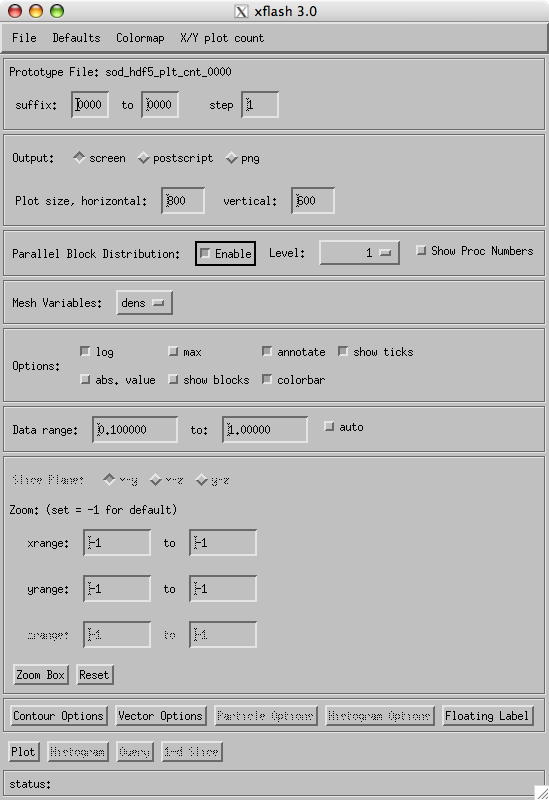
Now run IDL (idl or idl start_linux) and enter xflash3 at the IDL> prompt. You should see the main widget as shown in Figure 2.2.

Figure 2.2: The main xflash3 widget.

Select any of the checkpoint or plot files through the File/Open Prototype... dialog box. This will define a prototype file for the dataset, which is used by fidlr to set its own data structures. With the prototype defined, enter the suffixes '0000', '0005' and '1' in the three suffix boxes. This tells xflash3 which files to plot. xflash3 can generate output for a number of consecutive files, but if you fill in only the beginning suffix, only one file is read. Click the auto box next to the data range to automatically scale the plot to the data. Select the desired plotting variable and colormap. Under `Options,' select whether to plot the logarithm of the desired quantity and select whether to plot the outlines of the computational blocks. For very highly refined grids, the block outlines can obscure the data, but they are useful for verifying that FLASH is putting resolution elements where they are needed.

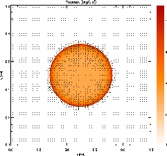
When the control panel settings are to your satisfaction, click the `Plot' button to generate the plot. For Postscript or PNG output, a file is created in the current directory. The result should look something like Figure 2.3, although this figure was generated from a run with eight levels of refinement rather than the five used in the quick start example run. With fewer levels of refinement, the Cartesian grid causes the explosion to appear somewhat diamond-shaped.

Figure 2.3: Example of xflash output for the Sedov problem with eight levels of refinement.

Please see Chp:FLASH IDL Routines (fidlr) for more information about visualizing FLASH output with IDL routines.

FLASH is intended to be customized by the user to work with interesting initial and boundary conditions. In the following sections, we will cover in more detail the algorithms and structure of FLASH and the sample problems and tools distributed with it.