29. Proton Emission Unit
Figure 29.1:
The Proton Emission unit directory tree.
|
|
When activated, the Proton Emission unit generates protons within the domain from nuclear fusion
reactions, follows the generated protons through the domain and detects them on specific detector screens.
Protons are deflected by Lorentz forces inside the domain due to presence of electric and magnetic
fields. The function ProtonEmission controls the generation and translation
of the protons inside the domain as well as their recording on the detector screens. For each cell in the domain
the average electric and magnetic fields are used and the electric and magnetic components do not change
within each cell. Each cell emits a certain number of protons (depending on temperature and fusion reaction
used) statistically inside a spherical cone characterized by an opening half-angle and a direction. The
half-angle of the emission cone can range between 0 and 180 degrees, the latter implying emission of the
protons into the complete surrounding sphere. For each detector an optional pinhole can be placed between
the domain and the detector screen. Currently the proton emission code assumes emission of protons without
altering the temperature and the chemical composition of the cell. This is an approximation valid only
for low reaction rates.
29.0.1 Proton Generation
Protons are generated by fusion reactions in domain regions of high temperature. Depending on the type
of nuclei present, several fusion reactions can take place in a cell. Currently there are two proton
generating fusion reactions implemented in FLASH:
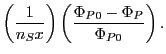
Nuclear reaction cross sections  are direct measures of probablity of nuclear reactions.
Let
are direct measures of probablity of nuclear reactions.
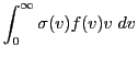
Let  be the initial flux of projectile nuclei P onto a homogeneous thin sheet of nuclei S
and
be the initial flux of projectile nuclei P onto a homogeneous thin sheet of nuclei S
and  the outcoming flux of projectile nuclei from the sheet. The flux of P is the number of P's
per unit area per unit time. The difference in flux
the outcoming flux of projectile nuclei from the sheet. The flux of P is the number of P's
per unit area per unit time. The difference in flux
 due to nuclear reactions
between P and S (there are other phenomena that lead to a reduction in flux, for example scattering) is the number
of reactions that happened in the sheet per unit area per unit time and is directly proportional to the
thickness
due to nuclear reactions
between P and S (there are other phenomena that lead to a reduction in flux, for example scattering) is the number
of reactions that happened in the sheet per unit area per unit time and is directly proportional to the
thickness  of the sheet, the initial flux of P's and the nuclei number density
  of S's in the sheet:
The proportionality constant  has dimensions of area and is defined as the nuclear reaction cross
section for S. Since always
has dimensions of area and is defined as the nuclear reaction cross
section for S. Since always
 , the dimensionless quantity
 denotes the probability of the nuclear reaction to happen in the sheet. The quantity
  can be viewed
as the number of S's per unit area of the sheet. Hence
can be viewed
as the number of S's per unit area of the sheet. Hence  is the area in the sheet covered by each S.
Rewriting the above equation we have:
is the area in the sheet covered by each S.
Rewriting the above equation we have:
The cross section of S is thus equal to the area of each S in the sheet times the probability of nuclear reaction
occuring in the sheet. It is thus the effective area of each S in the sheet that leads to a nuclear reaction.
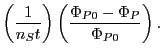
is dependent on the relative velocity of each P towards the S's in the sheet. Let us denote this velocity
by  and let us further consider only sheet sections in which all incident P's have the same . The sheet
thickness will be traversed by each P in time
and let us further consider only sheet sections in which all incident P's have the same . The sheet
thickness will be traversed by each P in time  and we have
  . Substituting this into the above
expression for and rearranging gives:
. Substituting this into the above
expression for and rearranging gives:
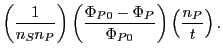
The quantity
 is called the reactivity of S and represents the probability of reaction per
unit density of S per unit time in the sheet. Let us multiply the expression on the r.h.s. by
is called the reactivity of S and represents the probability of reaction per
unit density of S per unit time in the sheet. Let us multiply the expression on the r.h.s. by  , where
 is the number density of incident P's onto the sheet. We have, after grouping together:
The quantity
 represents the number of P's in the sheet that reacted per volume unit
per time unit. It is known as the volumetric reaction rate between P and S (number of reactions per volume per time)
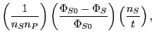
in the sheet. If we swap the particles with the target nuclei in the sheet, i.e. if we consider the P's stationary
in the sheet and the S's moving in the opposite direction, then is the same and we have:
represents the number of P's in the sheet that reacted per volume unit
per time unit. It is known as the volumetric reaction rate between P and S (number of reactions per volume per time)
in the sheet. If we swap the particles with the target nuclei in the sheet, i.e. if we consider the P's stationary
in the sheet and the S's moving in the opposite direction, then is the same and we have:
where now  refers to the flux of S's in the opposite direction. The volumetric reaction rate
  between
P and S must be identical in both pictures, hence:
between
P and S must be identical in both pictures, hence:
and therefore the nuclear cross sections
 and
and
 are equal and will be referred to as
the nuclear reaction cross section
are equal and will be referred to as
the nuclear reaction cross section  . The volumetric reaction rate is
where is the relative velocity between P's and S's. This equation allows for a comparison to reaction
rates of 2nd order chemical reactions. The number densities and of the nuclei play the role of
concentrations of reactants. The quantity
 is analogous to the chemical reaction constant, which in case
of nuclear reactions depends on the approach velocity of the nuclei and their effective interaction area. If both
nuclei P and S are the same, then using both and separately in the rate equation would overcount
the number of reactions by 2. If there are
is analogous to the chemical reaction constant, which in case
of nuclear reactions depends on the approach velocity of the nuclei and their effective interaction area. If both
nuclei P and S are the same, then using both and separately in the rate equation would overcount
the number of reactions by 2. If there are  identical nuclei in a certain volume, one can only form
 distinct pairs, which for large becomes
 . The volumetric reaction rate including
the possibility for identical nuclei reads
. The volumetric reaction rate including
the possibility for identical nuclei reads
where
 is 1, if P and S are identical and 0 elsewhere.
In a cell with a definite temperature  , the relative velocities between the interacting nuclei vary and
one must use a velocity distribution function
, the relative velocities between the interacting nuclei vary and
one must use a velocity distribution function  (most common used is Maxwellian). The volumetric nuclear
reactivity
must therefore be replaced by an averaged reactivity
(most common used is Maxwellian). The volumetric nuclear
reactivity
must therefore be replaced by an averaged reactivity
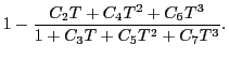
and the volumetric reaction rate becomes
The dimensions of
 are usually given in cm
 s
s .
It can be calculated from experimentally determined cross sections assuming a Maxwellian
velocity distribution of the nuclei at a certain temperature and integrating over the entire velocity
range. Since these integrations are time consuming, the values of
as a
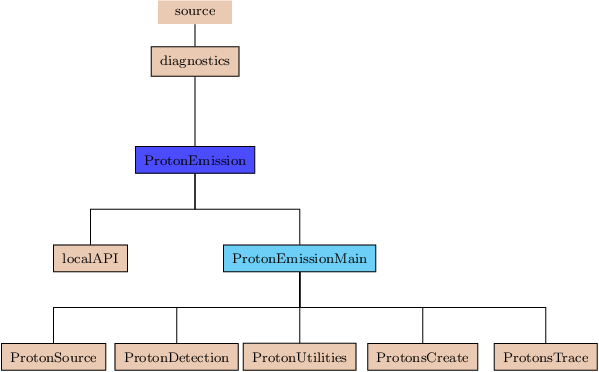
function of temperature are conveniently fitted using simple functional forms. For both above reactions,
FLASH uses the functional fit as provided by Bosch and Hale (1992):
.
It can be calculated from experimentally determined cross sections assuming a Maxwellian
velocity distribution of the nuclei at a certain temperature and integrating over the entire velocity
range. Since these integrations are time consuming, the values of
as a
function of temperature are conveniently fitted using simple functional forms. For both above reactions,
FLASH uses the functional fit as provided by Bosch and Hale (1992):
where
The values of the coefficients from  through
  and the valid temperature range of the fit
can be found in Atzeni and Meyer-Ter-Vehn (2004).
and the valid temperature range of the fit
can be found in Atzeni and Meyer-Ter-Vehn (2004).
The tracing of the protons through the domain is analogous to the one used for proton imaging. Currently
only  pairs are recorded for each proton on each detector screen. Time resolved proton emission is
not yet implemented, i.e. the protons exit the domain in one time step once they are created.
pairs are recorded for each proton on each detector screen. Time resolved proton emission is
not yet implemented, i.e. the protons exit the domain in one time step once they are created.
29.0.2 Proton Detector Screens
The setup of the proton detector screens and the proton recording technique is the same as for the proton
imaging unit (section 28.0.4). Option for additional pinholes is provided as well.
As there are no beams in this unit, the protons are recorded on the nearest detector screen in 3D space.
If protons do not hit any detector screen, they will be lost. As the protons are not associated with a
particular beam and detector, there is no option for recording offscreen protons.
29.0.3 Proton Emission Boxes
In order to allow for more simulation flexibility, the proton emission code is equipped with the possibility
of selecting active proton emission regions (boxes) inside the domain. If no such boxes are specified, the
entire domain is active, i.e. protons will be generated from the entire domain. If one or more emission boxes
are given, protons will only be generated from inside the box. Proton emission boxes are allowed to overlap
in space, but are not allowed to be completely outside the domain boundaries. Each emission box is characterized
by its rectangular bounding box coordinates (lower left and upper right corners).
To include the use of the Proton Emission unit, the following should be included into the
setup line command:
+protonEmission [pem_maxDetectors=<number> pem_maxEmissionBoxes=<number> threadProtonTrace=True]
- pem_maxDetectors: The maximum number of proton emission detectors for the simulation.
- pem_maxEmissionBoxes: The maximum number of proton emission boxes for the simulation.
- threadProtonTrace: Enables threading during proton domain tracing.
The runtime parameters for the proton emission unit are very similar to those for the proton imaging.
Setup and placement of detector parameters are identical to the proton imaging detectors.
The following are the runtime parameters for the proton emission detectors. The _n at the
end of each runtime parameter characterizes the detector number.
The following are the runtime parameters for the proton emission boxes. The _n at the
end of each runtime parameter characterizes the emission box number.
- pem_appendOldDetectorFiles: If set to true, emission protons will be added
to old existing detector files, provided old and new detector file names match.
- pem_cellStepTolerance: This factor times the smallest dimension of each cell is
taken as the positional error tolerance for the protons during their path (parabolic or Runge-Kutta)
tracing through each cell.
- pem_cellWallThicknessFactor: Controls the (imaginary) thickness of the cell
walls to ensure computational stability of the proton emission code. The cell thickness is defined as this
factor times the smallest cell dimension along all geometrical axes. The factor is currently
set to
 and should only very rarely be changed.
- pem_detailedTiming: If set to true, detailed timing info for several stages
during the proton emission will be provided in the application logfile.
- pem_detectorFileNameTimeStamp: If set to true, a time stamp will be added to
each detector file name. This allows for time splitting of detectors.
- pem_detectorXYwriteFormat: Controls formatted ascii output of the proton
pairs on the detector screens (default 'es20.10').
- pem_emissionAmplificationFactor: Amplifies the proton emission count of each
cell by this factor.
- pem_emissionConeHalfApexAngle: The half apex angle (degrees) of each cell emission
cone.
- pem_emissionConeCenter[X,Y,Z]: The global 3D components of the emission cone
center. This is for directional purposes only. Each cell sends an emission cone with the specified
half appex angle to this center location.
- pem_ignoreElectricalField: If true, the electrical field in each cell is ignored.
- pem_ignoreMagneticField: If true, the magnetic field in each cell is ignored.
- pem_maxProtonCount: The maximum number of emitted protons that can be
created on one processor per batch in the domain.
- pem_opaqueBoundaries: If true, the protons do not go through cells marked as
opaque boundaries.
- pem_printDetectors: If true, it prints detailed information about the proton
detectors to a file with name
 basename
 ProtonEmissionDetectors.txt, where basename is
the base name of the simulation.
ProtonEmissionDetectors.txt, where basename is
the base name of the simulation.
- pem_printMain: If true, it prints general information regarding the proton
emission setup to a file with name basenameProtonEmissionMain.txt, where basename
is the base name of the simulation.
- pem_printProtons: If true, it prints detailed information about the all protons
generated during the simulation. Protons are 'generated' on the domain surface and the info is written
to several files labeled by batch number BID, processor rank number PID and a time stamp. Each processor
writes its own file(s) with name(s): basenameprintProtonsBatchBIDProcPID.txt, where
basename is the base name of the simulation. Use of this feature is reserved ONLY for debugging
purposes and is currently limited to 10 batches and 100 processors per time stamp. Usage of a larger
number of batches/processors during a simulation does not abort the run, but protons on batches with
BID
 and processors with PID
  are simply ignored and not printed. Users other than code
developers should not activate this feature.
are simply ignored and not printed. Users other than code
developers should not activate this feature.
- pem_printProtonSources: If true, it prints general information regarding the proton
emission setup to a file with name basenameProtonEmissionMain.txt, where basename
is the base name of the simulation.
- pem_protonDeterminism: If true, the Grid Unit will be forced to use the sieve
algorithm to move the proton particle data. Forcing this algorithm will result in a slower movement
of data, but will fix the order the processors pass data and eliminate round off differences in
consecutive runs.
- pem_RungeKuttaMethod: Specifies which Runge Kutta method to use for proton tracing.
Current options are: 'CashKarp45' (order 4, default), 'EulerHeu12' (order 1), 'BogShamp23' (order 2),
'Fehlberg34' (order 3) and 'Fehlberg45' (order 4).
- pem_screenProtonBucketSize: Sets the bucket size for flushing screen protons
out to disk.
- pem_useParabolicApproximation: If true, the code traces protons parabolically through
cells for low
 / high combinations (section 28.0.1.2).
- useProtonEmission: If false, no proton emission will be performed,
even if the code was compiled to do so. Bypasses the need to rebuild the code.
- threadProtonTrace: If true, proton tracing through a block is threaded. This runtime
parameter can only be set during setup of the code.
Subsections