28. Proton Imaging Unit
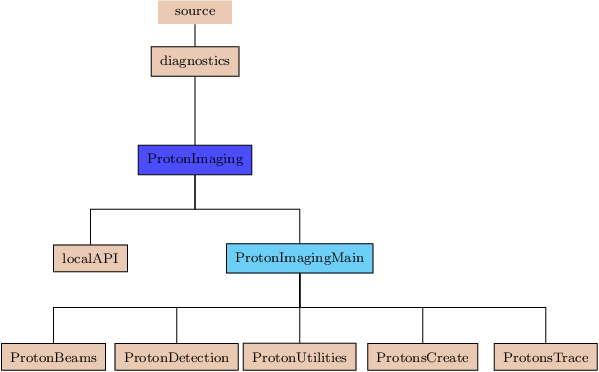
Figure 28.1:
The Proton Imaging unit directory tree.
|
|
The Proton Imaging unit fires proton beams onto the simulation domain and records their deflection
due to electric and magnetic fields on detector screens. The function ProtonImaging
is the main driver that orchestrates the proton imaging execution. The deflections
of the protons are calculated using the Lorentz force. For each cell in the domain
the average electric and magnetic fields are used and the electric and magnetic components do not change
within each cell. The code allows for setting up several proton beams with possibly different activation times
and several detector screens. Each beam is associated with only one detector, but a detector is allowed to
record the protons coming from more than one beam. This way one can simulate multienergetic proton beams by
splitting them into several computational beams with identical spatial (isospatial) specifications and identical
detector target but using different proton energies. Stacked film detectors for resolving different energy
components can be simulated by associating separate isospatial detectors to each energy component of multienergetic
proton beams. The mapping 'beam
 many detectors' is currently not allowed.
Tracing of the protons through the domain can be done in two ways: 1) crossing the domain during one time step
or 2) allowing for time resolved proton tracing, i.e. tracing the protons through the domain during many time
steps, if the velocities of the protons are sufficiently small. Although the proton imaging driver can be called
during an entire simulation with proton beams being activated at certain simulation times, it is highly
recommended to apply the proton imaging diagnostic as a post processing application on existing checkpoint
files. Screen protons can be appended to existing detector files, but the proton imaging code does not write
currently any data to the checkpoint files. Restarting a FLASH application from a previous proton imaging run
is hence not recommended, especially if the time resolved proton imaging version is used. Old disk protons
waiting to be transported though the domain may be out of sync when restarting a previous run.
28.0.1 Proton Deflection by Lorentz Force
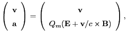
In the presence of an electric and magnetic field, the (relativistic and non-relativistic) Lorentz force in
CGS units on a proton in motion is:
where  is the charge of the proton in esu (g
 cm
cm s
s ),
),  the force
in dyne (g cm s
the force
in dyne (g cm s ),
),  the proton velocity (cm s),
  the speed of light
(
the speed of light
(
 cm s) and
  and
and  are the electric and magnetic
fields in Gauss (g cm
are the electric and magnetic
fields in Gauss (g cm s). The non-relativistic acceleration the proton experiences is:
where  is the mass rescaled charge
  of the proton. For uniform fields in each cell (constant
 and
and
 ), this leads to a set of 1st order coupled differential
equations in time
), this leads to a set of 1st order coupled differential
equations in time
for the velocity components  ,
,  and
and  . Given the initial proton
velocity components
. Given the initial proton
velocity components
 at time
  , the analytical solution to
this system of coupled differential equations becomes (assuming
, the analytical solution to
this system of coupled differential equations becomes (assuming  ):
):
where  is the magnitude of the magnetic field vector and
  and
and  are
the magnetic field magnitude rescaled magnetic and electric field components. The operator
are
the magnetic field magnitude rescaled magnetic and electric field components. The operator
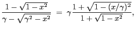
![$ [x\rightarrow y, y\rightarrow z, z\rightarrow x]$](img2546.png) stands for 'replace x with y, y with z and z with x'
in the formula for . In case
stands for 'replace x with y, y with z and z with x'
in the formula for . In case  ,
these equations reduce to:
,
these equations reduce to:
 ,
,
 and
and
 . Note that the units
of
. Note that the units
of  are the same as velocity. The quantities
  ,
,  and
and  are dimensionless.
Integrating , and over
are dimensionless.
Integrating , and over  , we get expressions for the positions
 ,
,  and
and  as a function of time. The resulting equations have terms involving
,
as a function of time. The resulting equations have terms involving
,  ,
,
![$ \cos[BQ_mt/c]$](img2559.png) and
and
![$ \sin[BQ_mt/c]$](img2560.png) , and cannot be solved analytically. We therefore resort
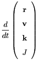
to a Runge-Kutta integration approach with the 6-dimensional ODE vector:
, and cannot be solved analytically. We therefore resort
to a Runge-Kutta integration approach with the 6-dimensional ODE vector:
For certain orientations of and , however, analytical solutions for
 and are possible (see the unit test section).
28.0.1.1 Relativistic Proton Equation of Motion
We state here briefly the relativistic proton equation of motion. Starting from the Lorentz equation
28.1, the force is the time derivative of the relativistic momentum  :
:
where  is the rest mass of the proton and
 is the Lorentz factor:
Performing the differentiation on the r.h.s. of Eq.(28.10) using the chain rule
(since both and thus  depend on time), we arrive at:
where
 and
and
 are the parallel and perpendicular components
of the acceleration
are the parallel and perpendicular components
of the acceleration
 with respect to the velocity vector:
 |
|
|
(28.13) |
Inverting Eq.(28.12) to find the acceleration from the force on a moving
proton leads to:
with magnitude:
and inserting the Lorentz force equation 28.1 we get the relativistic expression
for the acceleration:
where
 is the relativistic mass rescaled charge
 of the proton.
Comparing this expression with its non-relativistic version from Eq.(28.2),
the main difference is not only the relativistic increase in mass (
of the proton.
Comparing this expression with its non-relativistic version from Eq.(28.2),
the main difference is not only the relativistic increase in mass (
 ) but also an
extra term of order
) but also an
extra term of order  involving the electric field. The relativistic analytical velocity
solutions corresponding to Eqs.(28.6-28.8) are much more complicated and involve extra
logarithmic velocity component terms due to the extra relativistic velocity term.
involving the electric field. The relativistic analytical velocity
solutions corresponding to Eqs.(28.6-28.8) are much more complicated and involve extra
logarithmic velocity component terms due to the extra relativistic velocity term.
28.0.1.2 Approximate Solutions to the Non-Relativistic Proton Equation of Motion
Since Runge-Kutta integration with constraints (due to the cell boundaries) is expensive, we wish
to derive conditions under which the proton path through a cell approximates a parabola, for which
quadratic solutions to the path positions become available. To this end we expand
 in terms of around the cell entry point . We get:
where
are the acceleration and jerk vectors at the cell entry point. Integration of Eq.(28.18)
yields the path equation:
The leading parabolic error term is hence the term involving the jerk vector. The largest parabolic error
term  can be estimated by:
If is less than the allowed positional error of the computation, the parabolic approximation
is used. To get also the velocity components with the same accuracy, the jerk terms are used to
compute the velocities. If the jerk terms are omitted from the velocity calculations, the velocity
components would only be accurate to first order in and considerable error in velocity directions
can accumulate during a proton imaging application.
In order to get a feeling for the conditions under which the parabolic approximation is applied in
FLASH, let us first state the expression for the jerk vector  , which is obtained by noting
that
, which is obtained by noting
that
 and using the acceleration vector expression twice:
The maximum magnitude that the vector can achieve is given by the situation in which
the pairs
 and
and
 are perpendicular and
 is opposite to
  . This leads to
and the inequality will also hold for the individual components of . Assuming no electric
field, we can estimate the magnitude of for which the parabolic approximation should be valid.
In FLASH, the positional error is defined as a fraction  times the minimum cell side size.
For a cubic cell with sides
times the minimum cell side size.
For a cubic cell with sides  we can set up the parabolic condition on as follows:
The time it takes to cross the cubic cell is of the order of
 and we conservatively
extend this time by the factor of
and we conservatively
extend this time by the factor of
![$ \sqrt[3]{6}$](img2605.png) to get rid of the 6 in the denominator. The parabolic
condition on becomes
to get rid of the 6 in the denominator. The parabolic
condition on becomes
For typical FLASH runs, we have for 20MeV protons
 and is of the order of microns
(
and is of the order of microns
( cm) for typical simulations. The accuracy fraction is typically
  . We also
have
. We also
have
 and
and
 . Hence under these conditions we have:
i.e., all magnetic fields under  Gauss in a cell can be treated parabolically.
28.0.1.3 Approximate Solutions to the Relativistic Proton Equation of Motion
This follows along the lines of the previous section (28.0.1.2).
Eq.(28.19) must be replaced by the relativistic expression from
Eq.(28.16), replacing by , and Eq.(28.20)
must be replaced by the time derivative of Eq.(28.16),
replacing in the final expression by and  by
by  :
:
where
is equal to
 . Note the extra terms of order when compared
with Eqs.(28.19) and (28.20). The largest parabolic error expression in
Eq.(28.22) remains the same. Assuming again no electric field, the same steps
leading to the non-relativistic parabolic condition in Eq.(28.26), leads to:
. Note the extra terms of order when compared
with Eqs.(28.19) and (28.20). The largest parabolic error expression in
Eq.(28.22) remains the same. Assuming again no electric field, the same steps
leading to the non-relativistic parabolic condition in Eq.(28.26), leads to:
the only difference being in using the relativistic mass rescaled proton charge. For the 20MeV protons
this would lead to a factor of
 larger than in
Eq.(28.27), due to the relativistically reduced magnitude of .
larger than in
Eq.(28.27), due to the relativistically reduced magnitude of .
28.0.2 Setting up the Proton Beam
The setup of each proton beam follows closely the setup of the laser beams in 18.4.6.
The major difference is that the proton imaging beams originate from 3D capsules instead of 2D planar crossection
areas. This allows for simulating proton capsule aberrations in the proton beams. The radius of the capsule
as well as its center location is specified for each beam at runtime, as well as each beams full conical aperture
angle. Target coordinates are only needed for directional purposes and the target area is circular and perpendicular
to the beam's direction. Additional runtime parameters needed for each beam are: 1) the launching time (the beam
fires once the simulation time exceeds the launching time), 2) its target detector screen and 3) the number of
protons to be launched and their energies. Once each beam has been set up, it is checked, if its capsule
volume is completely outside of the computational domain. A beam capsule (partially) inside the domain is not
allowed. A local set of 3D rectangular grid unit vectors  ,
, ,
, is constructed for
each beam, such that points from the capsule center to the target center and
is constructed for
each beam, such that points from the capsule center to the target center and
 . The 3D grid unit vectors serve for generating statistical 3D points inside
the spherical capsule as well as statistical 2D points inside the circular target area.
. The 3D grid unit vectors serve for generating statistical 3D points inside
the spherical capsule as well as statistical 2D points inside the circular target area.
28.0.3 Creating the Protons
The protons inside each beam are created by connecting one-to-one the statistical 3D grid points inside the
capsule with the statistical 2D grid points inside the circular target area. The proton directions inside
each beam are therefore not conically collinear and are allowed to cross. The proton initial positions and
velocities on the domain surface are calculated using the same strategy as presented in
18.4.7.6. Protons missing the domain can either be simply ignored or directly
recorded on the detector screen.
28.0.3.1 Moving Protons through the Domain
As the total number of protons generated can be very large, special techniques have to be used to
overcome the computational memory constraints. The Proton Imaging unit has been designed to work
with a proton batch and screen proton bucket combination. Both the batch and the bucket are of much
smaller size than the total protons and screen protons generated and can be seen as temporary storage
devices for both entities.
During a time step, the active proton beams start filling the generated protons into the beam proton batch.
Once filled, the beam protons in the batch are sent through the domain, where they are either collected as
disk protons into the disk proton batch (if time resolved proton imaging was requested) or as screen
protons into the screen proton bucket. If the screen proton bucket is full, its contents (screen protons)
are written to the corresponding detector files and emptied. The refilling of both the beam/disk proton
batch and the screen bucket are independent of each other and both batch and bucket can be of different sizes.
The main function ProtonImaging processes beam/disk proton batch after batch
until no more active beam/disk protons are present. As an example, if at a time step we have 3 active
beams with  protons each and the dimension of the proton batch is set to
  , a total of
30 beam proton batches will be generated and sent through the domain.
, a total of
30 beam proton batches will be generated and sent through the domain.
28.0.3.2 Proton Specifications
Each beam/disk proton needs to know its position  and velocity
 as it traverses the domain.
In addition to these 6 components it needs to know: 1) the time spent travelling in domain, 2) the current
block and processor numbers, 3) a global identification tag, 4) the originating beam and target detector numbers.
Screen protons on the other hand are only defined on the detector screen and hence need no specific information
for domain travelling. Their information is reduced to a screen position coordinate pair
as it traverses the domain.
In addition to these 6 components it needs to know: 1) the time spent travelling in domain, 2) the current
block and processor numbers, 3) a global identification tag, 4) the originating beam and target detector numbers.
Screen protons on the other hand are only defined on the detector screen and hence need no specific information
for domain travelling. Their information is reduced to a screen position coordinate pair  and a detector number
to which detector they are associated with.
and a detector number
to which detector they are associated with.
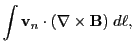
Additionally, upon request, the proton imaging code is able to calculate extra magnetic diagnostic
quantities  and
and  for each beam/disk and screen proton:
where
 denotes path integration, is the magnetic field vector and
 is the unit normal velocity vector along the proton path. Transforming the path integrals into
time integrals using the relation
is the unit normal velocity vector along the proton path. Transforming the path integrals into
time integrals using the relation
 , we get the differentials:
leading to extra 4 entries in the Runge-Kutta vector in Eq.(28.9):
If the parabolic path approximation is used for a cell, then
 , where
and are the velocity and acceleration at cell entry. For a cell contribution
we have (note this is a general result not depending on the parabolic approximation):
, where
and are the velocity and acceleration at cell entry. For a cell contribution
we have (note this is a general result not depending on the parabolic approximation):
where  is the cell crossing time and
  ,
,
 are the cell entry and exit locations of
the proton. For the parabolic cell contribution we have;
are the cell entry and exit locations of
the proton. For the parabolic cell contribution we have;
The parabolic path length integral can be solved exactly:
The second term is the offperpendicular and the third term the offcolinear contribution to the path
length. Taylor series expansion of this expression around in terms of the components of
gives the zeroth order term as
 corresponding to the path length for
 .
Likewise the zeroth order term for the expansion around in terms of the components of
is
.
Likewise the zeroth order term for the expansion around in terms of the components of
is
 which is the path length for
 . Application of the
above general formula must be done with some care to avoid computational pitfalls. The cases where
and are colinear must be handled separately. It is also easy to show,
for example, that for the offcolinear cases the natural logarithm argument is always
. Application of the
above general formula must be done with some care to avoid computational pitfalls. The cases where
and are colinear must be handled separately. It is also easy to show,
for example, that for the offcolinear cases the natural logarithm argument is always  .
.
28.0.4 Setting up the Detector Screens
Each detector screen is defined as a square planar area with a specific side length  and an optional
circular pinhole. The orientation of the screen in 3D space is specified by three components:
1) the center location of the screen
and an optional
circular pinhole. The orientation of the screen in 3D space is specified by three components:
1) the center location of the screen  , 2) the normal vector of the screen plane
  and 3) the
orthogonal unit vector pair
and 3) the
orthogonal unit vector pair  ,
, with origin at the center and oriented in such a way
that each unit vector is parallel to two opposite sides of the detector screen. Location of the pinhole
with origin at the center and oriented in such a way
that each unit vector is parallel to two opposite sides of the detector screen. Location of the pinhole
 is fixed by giving the distance between the two pinhole and detector centers and is always
located on the detector side opposite to . The circular pinhole area is coplanar to the detector
screen area.
While and are sufficient to characterize the screen plane, the exact location of the
detector square area is only specified once the orientation of (or ) is fixed.
For that purpose we define a tilting angle
is fixed by giving the distance between the two pinhole and detector centers and is always
located on the detector side opposite to . The circular pinhole area is coplanar to the detector
screen area.
While and are sufficient to characterize the screen plane, the exact location of the
detector square area is only specified once the orientation of (or ) is fixed.
For that purpose we define a tilting angle  of wrt one of the global 3D axes along
the normal vector . A tilting angle of
of wrt one of the global 3D axes along
the normal vector . A tilting angle of  would thus mean
that the chosen global axis and are coplanar.
would thus mean
that the chosen global axis and are coplanar.
28.0.4.1 Recording Protons on the Detector Screen
After each proton leaves the domain, it is located on the domain surface at a position  and
with (outward from domain) velocity . The goal is to see, if the proton actually hits the screen plane
and to record the local coordinates
and
with (outward from domain) velocity . The goal is to see, if the proton actually hits the screen plane
and to record the local coordinates  on the screen plane with coordinate basis
![$ [{\bf u}_x,{\bf u}_y]$](img2656.png) . After
some algebra we arrive at the following conditions
. After
some algebra we arrive at the following conditions
 |
 |
0 proton moves parallel to screen plane |
(28.39) |
 |
 |
0 proton hits screen plane |
(28.40) |
and the following expressions for the local coordinates
For better handling of the screen output data, the local coordinates are shifted and rescaled such that
![$ (x,y)\in [0,1]$](img2662.png) when the proton is on the detector screen. Using the detectors side length , we achieve
this by the following local coordinate transformation:
when the proton is on the detector screen. Using the detectors side length , we achieve
this by the following local coordinate transformation:
If a pinhole is present, the code has to check, if the proton makes it through the hole. Since the detector
screen area and the circular pinhole area are coplaner, we can use the local coordinate basis
located at the pinhole center to calculate a local pinhole coordinate
for each proton, in analogy to Eq.(28.41):
The proton makes it through the pinhole, if
 , where
  is the radius of the
pinhole.
is the radius of the
pinhole.
The user is able to specify via a runtime parameter, if he wants only the detector screen protons
to be written to the detector file or if he also wants to record the offscreen protons
![$ (x,y)\notin [0,1]$](img2672.png) .
Each detector file is currently an ascii file (formatted) and named:
.
Each detector file is currently an ascii file (formatted) and named:
| |
|
 |
(28.46) |
where  basename
 is the name of the simulation, detectorID is the detector number (currently
limited to the range [01-99]) and (optionally) timestamp is the simulation time when the file was created.
Only the pairs are written (first
is the name of the simulation, detectorID is the detector number (currently
limited to the range [01-99]) and (optionally) timestamp is the simulation time when the file was created.
Only the pairs are written (first  followed by
  on each line) without any headers. Thus the file
can be directly incorporated and read by other software for graphical output (see for example the proton
imaging ASCII
on each line) without any headers. Thus the file
can be directly incorporated and read by other software for graphical output (see for example the proton
imaging ASCII  PGM greyscale converter). Additionally, if requested, the detector file will contain
in columns 3 to 6 the proton magnetic diagnostic quantities
PGM greyscale converter). Additionally, if requested, the detector file will contain
in columns 3 to 6 the proton magnetic diagnostic quantities
 from Eqs.(28.31)
and (28.32), in that order.
from Eqs.(28.31)
and (28.32), in that order.
28.0.5 Time Resolved Proton Imaging
For some applications (slow moving protons, fast domain changing) it is desireable to adjust the domain
environment as the protons move through it. The proton imaging unit has been given this capability by
monitoring the time each proton spends in the domain and compare it to the computational time step. When
the proton time exceeds the time step value, it is stored as a disk proton which will be written to disk.
All disk protons from a previous time step must be first processed during a new time step before any new
beam protons are generated. During a time step, the main driver ProtonImaging
calls the following two tasks, each of which does the following operations:
Transport disk protons:
- Read all disk protons from old disk proton file
- Trace all disk protons through domain:
- To new disk proton file (if proton time time step)
- To screen detector
- Rename new disk proton file
 old disk proton file
Transport beam protons:
- Create all beam protons
- Trace all beam protons through domain:
- To new disk proton file (if proton time time step)
- To screen detector
- Append new disk proton file
old disk proton file
The time resolved application requires extra memory and disk storage due to the presence of disk protons as
well as extra reading/writing time from/to disk. If only a non-time resolved proton imaging run is requested,
the code skips all array allocations and operations associated with the disk protons, and only the underlined
actions of the transport beam protons task get activated.
To include the use of the Proton Imaging unit, the following should be included into the
setup line command:
+protonImaging [pi_maxBeams=<number> pi_maxDetectors=<number> threadProtonTrace=True]
- pi_maxBeams: The maximum number proton beams for the simulation.
- pi_maxDetectors: The maximum number of proton imaging detectors for the simulation.
- threadProtonTrace: Enables threading during proton domain tracing.
Using proton imaging runtime parameters in the flash.par file, the user can set up the proper proton
imaging configuration for his specific needs. The following list of runtime parameters is
currently available for the user.
The following are the runtime parameters for the proton imaging beams. The _n at the end of each
runtime parameter characterizes the beam number, hence replace _n by _1 for the first beam,
_n by _2 for the second beam, etc.
The following are the runtime parameters for the proton imaging detectors. As for the beams, the _n at the
end of each runtime parameter characterizes the detector number.
- pi_numberOfDetectors: The number of proton imaging detectors that are going to
be used.
- pi_detectorCenter[X,Y,Z]_n: The global 3D components of the detector center position
vector .
- pi_detectorNormal[X,Y,Z]_n: The local 3D components of the detector normal
vector .
- pi_detectorSideLength_n: The side length (cm) of the detector square screen.
- pi_detectorSideTiltingAngle_n: The tilting angle (degrees) of two sides
parallel to the detector screen unit axis
![$ {\bf u}_y]$](img2677.png) with respect to the tilting axis.
with respect to the tilting axis.
- pi_detectorSideTiltingAxis_n: The global tilting axis ('x','y' or 'z')
for the detector screen.
- pi_detectorAlignWRTbeamNr_n: A useful shortcut to place the detector
screen right along a beam path with the screen surface orthogonal to the beam path.
This, together with the specified detector distance from the beam capsule center, automatically calculates
the center vector and the normal vector . If a beam number
 is specified,
no alignment is performed and the user has to supply center vector and normal vector coordinates.
is specified,
no alignment is performed and the user has to supply center vector and normal vector coordinates.
- pi_detectorDist2BeamCapsule_n: The detector distance from the beam capsule center,
used only if the detector is alligned with respect to a beam.
- pi_detectorPinholeRadius_n: The radius of the pinhole. If no pinhole is used.
- pi_detectorPinholeDist2Det_n: The pinhole center distance from the detector center,
useful only if a pinhole radius
 was specified.
- pi_cellStepTolerance: This factor times the smallest dimension of each cell is
taken as the positional error tolerance for the protons during their path (parabolic or Runge-Kutta)
tracing through each cell.
- pi_cellWallThicknessFactor: Controls the (imaginary) thickness of the cell
walls to ensure computational stability of the proton imaging code. The cell thickness is defined as this
factor times the smallest cell dimension along all geometrical axes. The factor is currently
set to and should only very rarely be changed.
- pi_detectorFileNameTimeStamp: If set to true, a time stamp will be added to
each detector file name. This allows for time splitting of detectors.
- pi_detectorXYwriteFormat: Controls formatted ascii output of the proton
pairs on the detector screens (default 'es20.10').
- pi_detectorDGwriteFormat: Controls formatted ascii output of the magnetic
diagnostic quantities
 on the detector screens (default 'es15.5').
- pi_flagDomainMissingProtons: If true, any proton missing the domain will
abort the program. If false, protons missing the domain will be recorded directly on the detector
screen.
- pi_ignoreElectricalField: If true, the electrical field in each cell is ignored
and the proton movement is only governed by the magnetic field (deflection only).
- pi_IOaddDetectorScreens: If true, the square frame of each detector will be
added to the plotfile.
- pi_IOaddProtonsCapsule2Domain: If true, the proton paths from the capsule to
the domain entry point will be added to the plotfile.
- pi_IOaddProtonsDomain2Screen: If true, the proton paths from the domain exit
point to the detector screen will be added to the plotfile.
- pi_IOmaxBlockCrossingNumber: This is an estimate of the maximum proton path length
while travelling through the block. This estimate is given as an integer number in units of block sides
(default 5). Only in extremely rare cases, when the magnetic and electric fields are strong and sufficiently
warped inside a block and the protons start to circulate inside the block, does one have to increase
this number.
- pi_IOnumberOfProtons2Plot: The number of protons that are to be plotted and written
to the plotfile.
- pi_maxProtonCount: The maximum number of beam/disk protons that can be
created/read-in on one processor per batch in the domain.
- pi_opaqueBoundaries: If true, the protons do not go through cells marked as
opaque boundaries.
- pi_printBeams: If true, it prints detailed information about the proton
beams to a file with name basenameProtonBeamsPrint.txt, where basename is
the base name of the simulation.
- pi_printDetectors: If true, it prints detailed information about the proton
detectors to a file with name basenameProtonImagingDetectors.txt, where basename is
the base name of the simulation.
- pi_printMain: If true, it prints general information regarding the proton
imaging setup to a file with name basenameProtonImagingMainPrint.txt, where basename
is the base name of the simulation.
- pi_printProtons: If true, it prints detailed information about the all protons
generated during the simulation. Protons are 'generated' on the domain surface and the info is written
to several files labeled by batch number BID, processor rank number PID and a time stamp. Each processor
writes its own file(s) with name(s): basenameprintProtonsBatchBIDProcPID.txt, where
basename is the base name of the simulation. Use of this feature is reserved ONLY for debugging
purposes and is currently limited to 10 batches and 100 processors per time stamp. Usage of a larger
number of batches/processors during a simulation does not abort the run, but protons on batches with
BID
 and processors with PID
  are simply ignored and not printed. Users other than code
developers should not activate this feature.
are simply ignored and not printed. Users other than code
developers should not activate this feature.
- pi_protonDeterminism: If true, the Grid Unit will be forced to use the sieve
algorithm to move the proton particle data. Forcing this algorithm will result in a slower movement
of data, but will fix the order the processors pass data and eliminate round off differences in
consecutive runs.
- pi_recordOffScreenProtons: If true, protons not hitting their target detector screen
are also recorded on the detector files. These protons will have screen coordinate pairs
.
- pi_relativisticTracing: If true, the motion of the protons through the domain will
be treated relativistically using Eq.(28.16) for the relativistic acceleration
and Eq.(28.29) for the relativistic jerk terms.
- pi_RungeKuttaMethod: Specifies which Runge Kutta method to use for proton tracing.
Current options are: 'CashKarp45' (order 4, default), 'EulerHeu12' (order 1), 'BogShamp23' (order 2),
'Fehlberg34' (order 3) and 'Fehlberg45' (order 4).
- pi_screenProtonBucketSize: Sets the bucket size for flushing screen protons
out to disk.
- pi_screenProtonDiagnostics: If true, the magnetic diagnostic quantities
are evaluated for each proton and recorded on the detector screens.
- pi_timeResolvedProtonImaging: If true, it activates the time resolved proton
imaging part of the code. Protons might need several time steps to cross the domain.
- pi_useIOprotonPlot: If true, protons are plotted to the plotfile for visualization
pusposes.
- pi_useParabolicApproximation: If true, the code traces protons parabolically through
cells for low / high
 combinations (section 28.0.1.2).
- useProtonImaging: If false, no proton imaging will be performed,
even if the code was compiled to do so. Bypasses the need to rebuild the code.
- threadProtonTrace: If true, proton tracing through a block is threaded. This runtime
parameter can only be set during setup of the code.
The unit test for the proton imaging unit consists in sending a ring of protons perpendicular onto
either a uniform circular field or a radially outward uniform  field and measuring the deflection
(radial increase) of the ring as well as the magnitudes of the magnetic diagnostic quantities
field and measuring the deflection
(radial increase) of the ring as well as the magnitudes of the magnetic diagnostic quantities  and
from Eqs.(28.31) and (28.32). Due to the circular field or the radial
outward field, each proton experiences a radial outward force and the radial increase of the protons
can be calculated analytically. Exact analytical expressions for and are also possible.
and
from Eqs.(28.31) and (28.32). Due to the circular field or the radial
outward field, each proton experiences a radial outward force and the radial increase of the protons
can be calculated analytically. Exact analytical expressions for and are also possible.
Consider the case of a uniform circular magnetic field with constant magnetic flux density pointing
tangentially in clock- or anticlock-wise orientation around an axis, which we chose to be the
axis. If a proton has only a component velocity
 initially, then it will be deflected radially
outward or inward, depending on the clock- or anticlockwise orientation of . To simplify
the calculations, we assume that the proton is located on the positive axis, such that at this point we have
only a
initially, then it will be deflected radially
outward or inward, depending on the clock- or anticlockwise orientation of . To simplify
the calculations, we assume that the proton is located on the positive axis, such that at this point we have
only a  magnetic component, that is
  and
and  . Further we deal with the non-relativistic situation
first, as the extension to the relativistic case is trivial. We will use Eqs.(28.6-28.8)
for that purpose. Since no electric field is present, we have that:
. Further we deal with the non-relativistic situation
first, as the extension to the relativistic case is trivial. We will use Eqs.(28.6-28.8)
for that purpose. Since no electric field is present, we have that:
 |
|
0 |
(28.47) |
 |
|
 |
(28.48) |
 |
|
 |
(28.49) |
Putting these values into Eqs.(28.6-28.8), the proton velocities become:
 |
|
![$\displaystyle \pm v_{0y} \sin[BQ_mt/c]$](img2689.png) |
(28.50) |
 |
|
![$\displaystyle v_{0y} \cos[BQ_mt/c]$](img2690.png) |
(28.51) |
 |
|
0 |
(28.52) |
showing that the proton moves within the same -plane. The  sign in applies, if
  (anticlockwise orientation) and the
  sign, if
  (clockwise orientation). Integration over time
gives the position equations:
(clockwise orientation). Integration over time
gives the position equations:
Taking the anticlockwise orientation of , looking from above onto the fized -plane, the proton
will perform a half-circle of radius
 . We are interested in the (radial) deflection along
the axis. The proton will travel through the domain in the direction, where on exit the detector
screen is placed. If we place the detector right at the exit of the direction, then we can calculate
from the equation the time it takes for the proton to travel through (exit) the domain:
. We are interested in the (radial) deflection along
the axis. The proton will travel through the domain in the direction, where on exit the detector
screen is placed. If we place the detector right at the exit of the direction, then we can calculate
from the equation the time it takes for the proton to travel through (exit) the domain:
where  is the length of the domain in direction. If
 , then the proton will not
exit the domain but rather curve back inside the domain. This happens if either is too large (the domain
extends too far into the direction), is too large or the initial velocity
, then the proton will not
exit the domain but rather curve back inside the domain. This happens if either is too large (the domain
extends too far into the direction), is too large or the initial velocity  is too low.
For a given and , the limiting would be:
is too low.
For a given and , the limiting would be:
Inserting the  expression into the equation, we get:
The radial deflection  of the proton on the detector screen will be equal to
 and therefore:
The limiting radial deflection (i.e., the maximal radial deflection) that can be detected by the
screen at the domains exit is obtained by inserting the expression of  into the last
equation, which gets:
into the last
equation, which gets:
and is hence equal to the domains extension in direction.
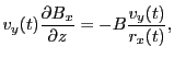
To evaluate the magnitude of the magnetic diagnostic quantities and , we start from the differential
equations derived from Eqs.(28.33) and (28.34):
where the first equation follows from the fact that the velocity magnitude does not change and the
second equation utilized the fact that for a proton positioned on the axis only the term
 from
from
 is nonzero (for anticlockwise rotation of we
have
is nonzero (for anticlockwise rotation of we
have
 ,
,  and
and
 , which gives at
  locations
 ). Performing the time integration
from to
). Performing the time integration
from to
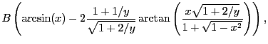
 and using the expressions for , and from
Eqs.(28.51), (28.53) and (28.56), we get:
and using the expressions for , and from
Eqs.(28.51), (28.53) and (28.56), we get:
where we have used the dimensionless quantities:
Since the electrical field is zero, inclusion of relativity into the deflection equations is trivial.
There is no increase in velocity as the proton travels inside the domain, which means that
stays constant. To account for relativistic effects, one simply has to replace in the radial deflection
and magnetic diagnostic equations by
, where
 .
For fixed parameters, the relativistic radial deflection is always less than the non-relativistic one.
This can be shown by evaluating the ratio between the two radial deflections. Using the non-relativistic
as defined in Eq.(28.65), we have:
.
For fixed parameters, the relativistic radial deflection is always less than the non-relativistic one.
This can be shown by evaluating the ratio between the two radial deflections. Using the non-relativistic
as defined in Eq.(28.65), we have:
and, since  and
and
 , it follows that:
In this section we state the radial deflection equations in the presence of a radial outward
directed electric field. To simplify again the calculations, we assume that the proton is located
such that at this point we have only a electric component, that is  and
and  .
To include the relativistic case, we start from the relativistic acceleration in
Eq.(28.16) and solve the set of differential equations corresponding
to the unit test setup:
.
To include the relativistic case, we start from the relativistic acceleration in
Eq.(28.16) and solve the set of differential equations corresponding
to the unit test setup:
with initial conditions
 and
and
 . The results are:
|
|
 |
(28.71) |
|
|
 |
(28.72) |
|
|
0 |
(28.73) |
where
is evaluated using
with
 for the non-relativistic case, and
  is 1 for the relativistic case and 0 otherwise. Integration
over time gives (note the relativistic corrections to the classical expressions):
is 1 for the relativistic case and 0 otherwise. Integration
over time gives (note the relativistic corrections to the classical expressions):
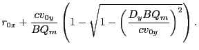
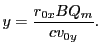
From the equation for we get the domain crossing time in the direction as:
and the resulting radial reflection
is:
In contrast to the magnetic field radial deflection, there is, for a fixed a certain
and for a fixed a certain , beyond which the relativistic radial deflection is greater
than the non-relativistic one. Using the simplification:
we have for the ratio:
But the function
 is a monotonic decaying function between
  for
for  and
and  for
for
 . Hence at some we must have
 , beyond which
we have
, beyond which
we have
 . The crossover radial deflecion
 ,
at which both the non-relativistic and the relativistic radial reflections coincide, can be calculated
by finding the solutions for
,
at which both the non-relativistic and the relativistic radial reflections coincide, can be calculated
by finding the solutions for  and
in the following two equations:
and
in the following two equations:
Note that the first equation, defining as a function of , cannot be solved analytically
and one must resort to numerical approaches.
We set up a 3D cartesian domain consisting of a rectangular box with dimensions (in cm):
axis ![$ [0,3]$](img2768.png) , axis
, axis ![$ [0,1]$](img1397.png) and axis . A circular beam of 10000 protons
with radius 0.5cm is shot along the axis perpendicular to the
and axis . A circular beam of 10000 protons
with radius 0.5cm is shot along the axis perpendicular to the  plane and centered
on the plane at (1.5,1.5). The square detector screen was placed extremely close to the
domain exit in direction and was of the same size as the domain's plane, i.e., of
side length 3cm and centered at (1.5,1.5). The variable parameters used were: 1) the proton
energies (currently only 20MeV), 2) the uniform refinement levels (3,4,5) and the magnetic / electric
fields (in Gauss). The following radial deflections were recorded: 1) the theoretical
plane and centered
on the plane at (1.5,1.5). The square detector screen was placed extremely close to the
domain exit in direction and was of the same size as the domain's plane, i.e., of
side length 3cm and centered at (1.5,1.5). The variable parameters used were: 1) the proton
energies (currently only 20MeV), 2) the uniform refinement levels (3,4,5) and the magnetic / electric
fields (in Gauss). The following radial deflections were recorded: 1) the theoretical
 , 2) the maximum
 , 3) the minimum
 and 4) the
average
and 4) the
average
 .
.
From the FLASH setup parameters, we can calculate the following values for 20 MeV protons:
Tables 28.1, 28.2 and 28.3 show the obtained FLASH
results for the radial deviation, the magnetic diagnostic value and the magnetic diagnostic magnitude,
including a run with .
Table:
Magnetic outward radial deflections: maximum
,
minimum
, average
and theoretical
from
Eq.(28.59) on a ring of 20 MeV protons for uniform domain refinement levels 3,4,5.
Subscript numbers indicate multiplication by negative exponents:  means
means
 .
The radial deflection values are in cm. Italic numbers represent the relativistic results.
.
The radial deflection values are in cm. Italic numbers represent the relativistic results.
| Proton energy 20 MeV (0.203 c), Refinement Levels = 3,4,5 |
|
|
|
|
|
 |
 |
 |
 |
|
| |
|
 |
 |
|
| |
|
 |
 |
|
| |
 |
 |
 |
|
| |
|
 |
 |
|
| |
|
 |
 |
|
|
 |
 |
 |
|
| |
|
 |
 |
|
| |
|
 |
 |
|
| |
 |
 |
 |
|
| |
|
 |
 |
|
| |
|
 |
 |
|
 |
 |
 |
 |
|
| |
|
 |
 |
 |
| |
|
 |
 |
|
| |
 |
 |
 |
|
| |
|
 |
 |
|
| |
|
 |
 |
|
Table:
Magnetic diagnostic values: maximum  ,
minimum
,
minimum  , average
  and theoretical
  from Eq.(28.64)
on a ring of 20 MeV protons for uniform domain refinement levels 3,4,5. Subscript numbers
indicate multiplication by positive exponents: means
from Eq.(28.64)
on a ring of 20 MeV protons for uniform domain refinement levels 3,4,5. Subscript numbers
indicate multiplication by positive exponents: means
 . All
values are in Gauss. Italic numbers represent the relativistic results.
. All
values are in Gauss. Italic numbers represent the relativistic results.
| Proton energy 20 MeV (0.203 c), Refinement Levels = 3,4,5 |
|
|
|
|
|
|
 |
 |
 |
|
| |
 |
 |
 |
 |
| |
 |
 |
 |
|
| |
 |
 |
 |
|
| |
 |
 |
 |
 |
| |
 |
 |
 |
|
|
 |
 |
 |
|
| |
 |
 |
 |
 |
| |
 |
 |
 |
|
| |
 |
 |
 |
|
| |
 |
 |
 |
 |
| |
 |
 |
 |
|
|
 |
 |
 |
|
| |
 |
 |
 |
 |
| |
 |
|
 |
|
| |
 |
 |
 |
|
| |
 |
 |
 |
 |
| |
 |
 |
 |
|
Table:
Magnetic diagnostic values: maximum  ,
minimum
,
minimum  , average
  and theoretical
  from Eq.(28.63)
on a ring of 20 MeV protons for uniform domain refinement levels 3,4,5. Subscript numbers
indicate multiplication by positive exponents: means
. All
values are in units of Gauss cm. Italic numbers represent the relativistic results.
from Eq.(28.63)
on a ring of 20 MeV protons for uniform domain refinement levels 3,4,5. Subscript numbers
indicate multiplication by positive exponents: means
. All
values are in units of Gauss cm. Italic numbers represent the relativistic results.
| Proton energy 20 MeV (0.203 c), Refinement Levels = 3,4,5 |
|
|
|
|
|
|
 |
 |
 |
|
| |
|
 |
 |
|
| |
|
|
|
|
| |
 |
 |
 |
|
| |
|
 |
 |
|
| |
|
|
|
|
|
 |
 |
 |
|
| |
|
 |
 |
|
| |
|
 |
 |
|
| |
 |
 |
 |
|
| |
|
 |
 |
|
| |
 |
 |
 |
|
|
 |
 |
 |
|
| |
|
 |
 |
|
| |
|
 |
 |
|
| |
 |
 |
 |
|
| |
|
 |
 |
 |
| |
|
 |
 |
|
From the FLASH setup parameters, we can calculate the following values for 20 MeV protons:
Table 28.4 shows the obtained FLASH results, including a run with  .
.
Table:
Electric outward radial deflections: maximum
,
minimum
, average
and theoretical
from Eq.(28.78) on a ring of 20 MeV protons for uniform domain refinement levels 3,4,5. Subscript
numbers indicate multiplication by negative exponents: means
. The radial
deflection values are in cm. Italic numbers represent the relativistic results.
| Proton energy 20 MeV (0.203 c), Refinement Levels = 3,4,5 |
|
|
|
|
|
|
 |
 |
 |
|
| |
|
 |
 |
|
| |
|
 |
 |
|
| |
 |
 |
 |
|
| |
|
 |
 |
|
| |
|
 |
 |
|
|
 |
 |
 |
|
| |
|
 |
 |
|
| |
|
 |
 |
|
| |
 |
 |
 |
|
| |
|
 |
 |
|
| |
|
 |
 |
|
 |
 |
 |
 |
|
| |
|
 |
 |
|
| |
|
 |
 |
|
| |
 |
 |
 |
|
| |
|
 |
 |
|
| |
|
 |
 |
|
Subsections
![$\displaystyle \frac{1}{\gamma({\bf v})m}\sqrt{F^2-\frac{1+\gamma({\bf v})^2}{c^2\gamma({\bf v})^2}
[{\bf v}\cdot {\bf F}]^2},$](img2575.png)
![$\displaystyle {\bf r}_0 + {\bf v}_0t + \frac{{\bf a}_0}{2}t^2 + \frac{{\bf j}_0}{6}t^3 + O[t^4].$](img2590.png)

![$\displaystyle \int^T_0 {\bf v}(t)\cdot (\nabla\times {\bf B}) dt =
\int^T_0 d{\...
...\times {\bf B}) =
\left[{\bf r}(T)-{\bf r}_0\right]\cdot (\nabla\times {\bf B})$](img2638.png)
![$\displaystyle +
\left.\frac{\vert{\bf a}_0\times {\bf v}_0\vert^2}{\vert{\bf a}...
...\bf a}_0\cdot {\bf v}_0+\vert{\bf a}_0\vert\vert{\bf v}_0\vert}\right)}\right].$](img2643.png)
![$\displaystyle \frac{{\bf u}_y\cdot [{\bf v}\times ({\bf H}-{\bf P})]}{{\bf v}\cdot {\bf n}}$](img2667.png)
![$\displaystyle \frac{{\bf u}_x\cdot [({\bf H}-{\bf P})\times {\bf v}]}{{\bf v}\cdot {\bf n}}.$](img2669.png)

![$\displaystyle r_{0x} + \frac{EQ_{m\gamma}t^2}{2}\left[2\left(\frac{EQ_{m\gamma}...
...
\left(\sqrt{1+\left(\frac{EQ_{m\gamma}t}{c}\right)^2}-1\right)\right]^{\delta}$](img2750.png)
![$\displaystyle r_{0y} + v_{0y}t\left[\left(\frac{EQ_{m\gamma}t}{c}\right)^{-1}\operatorname{arsinh}
\left(\frac{EQ_{m\gamma}t}{c}\right)\right]^{\delta}$](img2751.png)
![$\displaystyle \frac{D_y}{v_{0y}}\left[\left(\frac{D_yEQ_{m\gamma}}{cv_{0y}}\right)^{-1}
\sinh\left(\frac{D_yEQ_{m\gamma}}{cv_{0y}}\right)\right]^{\delta}$](img2752.png)


![$\displaystyle \frac{d{\bf p}}{dt} = \frac{d[\gamma({\bf v}) m{\bf v}]}{dt},$](img2564.png)
![$\displaystyle \frac{1}{\gamma({\bf v})m}\left({\bf F} - \frac{[{\bf v}\cdot {\bf F}]{\bf v}}{c^2}\right)$](img2573.png)
![$\displaystyle {\bf v}_0 + \left\vert\frac{d{\bf v}(t)}{dt}\right\vert _{t=0}t
+ \frac{1}{2}\left\vert\frac{d^2{\bf v}(t)}{dt^2}\right\vert _{t=0}t^2
+ O[t^3]$](img2583.png)
![$\displaystyle {\bf v}_0 + {\bf a}_0t + \frac{{\bf j}_0}{2}t^2 + O[t^3],$](img2584.png)


![$\displaystyle \frac{{\bf u}_y\cdot [{\bf v}\times ({\bf C}-{\bf P})]}{{\bf v}\cdot {\bf n}}$](img2660.png)
![$\displaystyle \frac{{\bf u}_x\cdot [({\bf C}-{\bf P})\times {\bf v}]}{{\bf v}\cdot {\bf n}}.$](img2661.png)

![$\displaystyle \frac{D_y^2EQ_{m\gamma}}{2v_{0y}^2}
\left[\left(\frac{D_yEQ_{m\ga...
...ght)^{-2}
\sinh^2\left(\frac{D_yEQ_{m\gamma}}{2cv_{0y}}\right)\right]^{\delta}.$](img2753.png)
