Subsections
34.4 Unit Tests
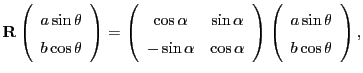
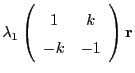
Consider the following ODE in 2D, operating on a 2D vector  :
:
This ODE describes a rotational ( ) and sheer (
 ) force on
a particle located at . If
) force on
a particle located at . If
 , then the ODE describes a
particle revolving in a circle of radius
, then the ODE describes a
particle revolving in a circle of radius
 , the initial radius of the particle.
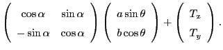
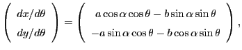
The general solution to the above ODE is:
, the initial radius of the particle.
The general solution to the above ODE is:
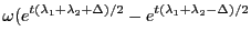
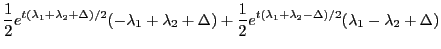
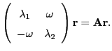
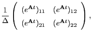
The matrix exponential is given by (using
 and
and
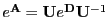 , where
  is diagonal):
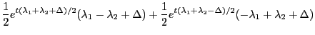
where
 |
 |
 |
(34.25) |
 |
|
 |
(34.26) |
 |
|
 |
(34.27) |
 |
|
 |
(34.28) |
and
For general values of
 , the path of the particle is a spiral around the
origin. Closed paths are possible, if at certain times
, the path of the particle is a spiral around the
origin. Closed paths are possible, if at certain times  we have
 .
A necessary condition is thus that the offdiagonal elements of
.
A necessary condition is thus that the offdiagonal elements of
 have to become zero
for certain . Since each of these elements has a factor of the structure
have to become zero
for certain . Since each of these elements has a factor of the structure  , then
either both
, then
either both  and
and  are real and equal or and are imaginary with oposite sign. Both
situations can only happen, if
are real and equal or and are imaginary with oposite sign. Both
situations can only happen, if
 . The first case (
 real and equal) is
only possible if
real and equal) is
only possible if  and the second case ( imaginary and of opposite sign) only if
 is imaginary. Hence, necessary conditions for a closed path are:
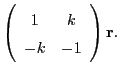
Let us now introduce the parameter  such that:
Then our closed path ODE becomes:
and, since  is now just merely a scaling factor, we can further condense the closed
path ODE to:
is now just merely a scaling factor, we can further condense the closed
path ODE to:
This is the 2D ellipse ODE we are going to use for our Runge Kutta test. Inserting
 ,
,
 and
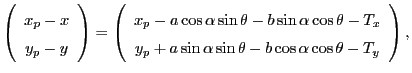
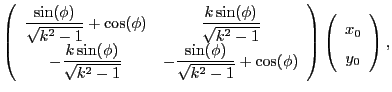
and  into the above general solution, we obtain, after inserting the identity
 , the following real path solution:
where
For
 , the 2x2 matrix is equal to
  , i.e. the particle made
a half revolution. For
, i.e. the particle made
a half revolution. For
 , the 2x2 matrix is equal to
  and
the particle made a complete revolution. The time
and
the particle made a complete revolution. The time  it takes for the particle to make one complete
revolution (its time period) is thus:
it takes for the particle to make one complete
revolution (its time period) is thus:
The square of the distance
![$ d^2=[x(t)]^2+[y(t)]^2$](img3469.png) the particle is found from the origin has a
minimum and a maximum at the following angles:
the particle is found from the origin has a
minimum and a maximum at the following angles:
 |
|
![$\displaystyle \arctan\left[\sqrt{\dfrac{k+1}{k-1}}\dfrac{x_0+y_0}{x_0-y_0}\right]$](img3471.png) |
(34.38) |
 |
|
![$\displaystyle -\arctan\left[\sqrt{\dfrac{k-1}{k+1}}\dfrac{x_0-y_0}{x_0+y_0}\right]$](img3473.png) |
(34.39) |
 |
|
 |
(34.40) |
 |
|
 |
(34.41) |
These angles (range
![$ [-\pi/2,+\pi/2]$](img3478.png) ) give only the angles to the nearest maximum/minimum point
from the original position
) give only the angles to the nearest maximum/minimum point
from the original position  . The other two angles corresponding to the remaining maximum/minimum
distance points are obtained by adding
. The other two angles corresponding to the remaining maximum/minimum
distance points are obtained by adding  . The corresponding times are:
The corresponding minimum and maximum square distances are:
where the signum function sgn is:
From these formulas we see that
- if
 and
and  , then the first
  is equal to zero, i.e. the particle is at its minimum
distance
is equal to zero, i.e. the particle is at its minimum
distance
 from the origin.
- if and
 , then the first
  is equal to zero, i.e. the particle is at its maximum
distance
from the origin.
is equal to zero, i.e. the particle is at its maximum
distance
from the origin.
- if
 and , then the first is equal to zero, i.e. the particle is at its maximum
distance
from the origin.
and , then the first is equal to zero, i.e. the particle is at its maximum
distance
from the origin.
- if and , then the first is equal to zero, i.e. the particle is at its minimum
distance
from the origin.
- the aspect ratio
 of the elliptical path is equal to
![$ A=\sqrt{(k+\mbox{sgn}[k])/(k-\mbox{sgn}[k])}$](img3499.png) .
.
We next develop the approach and formulas to find the minimum/maximum distance from a general
point in a 2D domain to a general ellipse inside this 2D domain.
34.4.1.2 Minimum and maximum distance from a point to a general ellipse in a 2D cartesian domain
We will first get the general parametric equation of an ellipse in 2D cartesian space. We start
by placing a 2D ellipse with its center at the cartesian origin and with its minor/major axis
aligned along the cartesian y/x axis. Let the semi-major axis have length  and the semi-minor
axis have length
and the semi-minor
axis have length  . The parametric equation for this ellipse is:
where the angle parameter is in the range
 . Next we clockwise rotate the entire
ellipse such that the minor axis makes an angle
. Next we clockwise rotate the entire
ellipse such that the minor axis makes an angle  with the cartesian y-axis. The range of this
rotation angle is
with the cartesian y-axis. The range of this
rotation angle is
 . The parametric equation for the rotated ellipse becomes
where  is the rotation matrix that sends every point to its new rotated point. Finally we add
the center translation vector
is the rotation matrix that sends every point to its new rotated point. Finally we add
the center translation vector
 to the equation for ellipses that are not located at
the cartesian origin:
to the equation for ellipses that are not located at
the cartesian origin:
This is the general parametric equation of any ellipse in 2D cartesian space. Consider a specific point
 on the ellipse. The tangent line at this ellipse point contains the tiny derivative vector
with its origin at the ellipse point . The other vector we consider is the vector
which also has its origin at the ellipse point . The minimum distance occurs for
those  for which
 (perpendicular vectors). This gives the following
equation for :
(perpendicular vectors). This gives the following
equation for :
where
Note, that  , whenever
  . For
. For  (a circle) we will have
  and the equation
becomes easily solvable. The elliptical
and the equation
becomes easily solvable. The elliptical  term makes the equation much harder to solve.
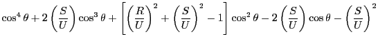
Eliminating the
term makes the equation much harder to solve.
Eliminating the
 term, we arrive at the following quartic equation in
 :
:
Its solutions give us up to 4 different possible angles . However, to each
solution there correspond two
solutions via
 ,
increasing the total possible solutions to 8. Each of these 8 solutions must be checked for
the minimum and maximum distance given by
,
increasing the total possible solutions to 8. Each of these 8 solutions must be checked for
the minimum and maximum distance given by  . As far as the number of real solutions
for the above quartic is concerned, when the point is inside or close to the ellipse, we can
visualize that there are 4 possible directions from the point to the ellipse for which we have
(i.e. we hit the ellipse curve at right angles). Hence for this point
location we expect 4 real quartic solutions. On the other hand, if we are far away from the ellipse,
only 2 such points on the elliptical curve will exist and we expect 2 real and 2 complex solutions.
We should never get 4 complex solutions of the above quartic.
. As far as the number of real solutions
for the above quartic is concerned, when the point is inside or close to the ellipse, we can
visualize that there are 4 possible directions from the point to the ellipse for which we have
(i.e. we hit the ellipse curve at right angles). Hence for this point
location we expect 4 real quartic solutions. On the other hand, if we are far away from the ellipse,
only 2 such points on the elliptical curve will exist and we expect 2 real and 2 complex solutions.
We should never get 4 complex solutions of the above quartic.
We will now set up the unit test for the Runge Kutta 2D ellipse test. We start by stating the
initial conditions and the requested shape of the ellipse:
- The particle is initially at position
 .
.
- We want the particle to follow an elliptical path with given aspect ratio .
From this requested aspect ratio we calculate our needed  as:
as:
and we take to be positive from now on. This means that the particle will start
moving along the elliptical curve in the clockwise direction. By looking at the general
formulas derived in the previous sections, we can state the following properties and
equations for the ellipse. The square distance extrema and locations will be:
From this we see that the major and minor semi-axis will have lengths:
From the particle's initial position at  , the minor and major semi-axis will be
reached at the following times (
, the minor and major semi-axis will be
reached at the following times (
 ):
):
Hence the period of one complete revolution (returning to ) is given by:
The ellipse is represented by the following two (equivalent) forms:
and the parametric time equations:
Each of the following Runge Kutta runs follows the elliptical curve through a full ellipse
revolution, starting at the initial at position
. The calculations are
stopped as soon as the  line is crossed once, with the last crossing point still included
in the calculation. Chosing an ellipse with an aspect ration of
line is crossed once, with the last crossing point still included
in the calculation. Chosing an ellipse with an aspect ration of  , we report
the following data using fractional errors of
, we report
the following data using fractional errors of
 and
and  and a coordinate error base vector of
 (Eq.(34.15) for each Runge Kutta run in separate tables:
- The embedded RK scheme used and its order.
- The number of RK steps used to trace the full elliptical curve.
- The overall largest RK step coordinate error
 , which should be
 .
.
- The maximum time distance error
 from the elliptical curve, where
is a measure of how far the RK curve deviates from the true elliptical curve at time  .
The quantity
.
The quantity  can be viewed as a global error of the RK scheme.
- The maximum of the closest distance error
 to the true elliptical curve.
The closest elliptical distance error
to the true elliptical curve.
The closest elliptical distance error
 is calculated using the approach outlined
in section 34.4.1.2 and is a measure of how closely the RK scheme
traces out the true elliptical curve.
is calculated using the approach outlined
in section 34.4.1.2 and is a measure of how closely the RK scheme
traces out the true elliptical curve.
Table 34.1 shows the obtained FLASH results. The higher order Fehlberg (5) and Cash-Karp (5)
RK schemes outperform the lower order ones. The Cash-Karp RK scheme gives the best performance and is thus
the set default RK scheme for the Runge Kutta unit.
Table 34.1:
Number of RK steps, largest RK step coordinate error
,
maximum time distance error
and maximum closest distance error
values
for a complete RK elliptical curve tracing with amplification , starting at the point
.
Results shown as a function of embedded RK scheme used with fractional errors
and
 .
.
| RK scheme (order) |
RK steps |
|
|
|
| Fractional error
|
| Euler-Heun (2) |
67887 |
 |
 |
 |
| Bogacki-Shampine (3) |
1102 |
 |
 |
 |
| Fehlberg (4) |
228 |
 |
 |
 |
| Fehlberg (5) |
84 |
 |
 |
 |
| Cash-Karp (5) |
60 |
 |
 |
 |
| Fractional error
|
| Euler-Heun (2) |
6788695 |
 |
 |
 |
| Bogacki-Shampine (3) |
23729 |
 |
 |
 |
| Fehlberg (4) |
2272 |
 |
 |
 |
| Fehlberg (5) |
526 |
 |
 |
 |
| Cash-Karp (5) |
372 |
 |
 |
 |
A binomial homogeneous ODE is an ODE of the form ( ):
):
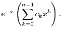
whose general solution is
We are interested in the particular solution with
 :
:
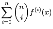
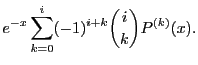
The derivatives of this particular solution are given by:
The values of the -th derivative of  at
at  are the factorials of , i.e. we
have
are the factorials of , i.e. we
have
 . Thus the inital set of conditions at for the particular
solution are:
. Thus the inital set of conditions at for the particular
solution are:
where  denotes the number of out-of-place permutations (derangements, no numbers in original places)
of
denotes the number of out-of-place permutations (derangements, no numbers in original places)
of  . A recursive formula for can be given:
![$ !i=(i-1)[!(i-1)+!(i-2)]$](img3600.png) , with starting values
, with starting values  and
and  . Note that the given set of initial condition implies
due to the definition of the binomial ODE equation.
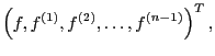
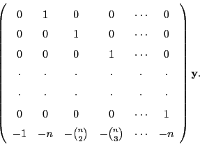
To solve the binomial ODE using the Runge Kutta scheme, the usual transformation to a set of coupled
1st order ODE's is done. Define the  -dimensional vector
the coupled set of 1st order ODE's are in matrix form:
We compare the Runge Kutta vector  with the vector evaluated using Eq.(34.73).

![$\displaystyle \dfrac{k(x_0^2+y_0^2)+2x_0y_0}{k+\mbox{sgn}[k]}$](img3485.png)
![$\displaystyle \dfrac{k(x_0^2+y_0^2)+2x_0y_0}{k-\mbox{sgn}[k]},$](img3487.png)