Next: 18.2 Ionization Unit Up: 18. Local Source Terms Previous: 18. Local Source Terms Contents Index
The nuclear burning implementation of the Burn unit uses a sparse-matrix semi-implicit ordinary differential equation (ODE) solver to calculate the nuclear burning rate and to update the fluid variables accordingly (Timmes 1999). The primary interface routines for this unit are Burn_init, which sets up the nuclear isotope tables needed by the unit, and Burn, which calls the ODE solver and updates the hydrodynamical variables in a single row of a single block. The routine Burn_computeDt may limit the computational timestep because of burning considerations. There is also a helper routine Simulation/SimulationComposition/Simulation_initSpecies (see Simulation_initSpecies) which provides the properties of ions included in the burning network.
Modeling thermonuclear flashes typically requires the energy generation rate due to nuclear burning over a large range of temperatures, densities and compositions. The average energy generated or lost over a period of time is found by integrating a system of ordinary differential equations (the nuclear reaction network) for the abundances of important nuclei and the total energy release. In some contexts, such as supernova models, the abundances themselves are also of interest. In either case, the coefficients that appear in the equations are typically extremely sensitive to temperature. The resulting stiffness of the system of equations requires the use of an implicit time integration scheme.
A user can choose between two implicit integration methods and two linear algebra packages in FLASH. The runtime parameter odeStepper controls which integration method is used in the simulation. The choice odeStepper = 1 is the default and invokes a Bader-Deuflhard scheme. The choice odeStepper = 2 invokes a Kaps-Rentrop or Rosenbrock scheme. The runtime parameter algebra controls which linear algebra package is used in the simulation. The choice algebra = 1 is the default and invokes the sparse matrix MA28 package. The choice algebra = 2 invokes the GIFT linear algebra routines. While any combination of the integration methods and linear algebra packages will produce correct answers, some combinations may execute more efficiently than others for certain types of simulations. No general rules have been found for best combination for a given simulation. The most efficient combination depends on the timestep being taken, the spatial resolution of the model, the values of the local thermodynamic variables, and the composition. Users are advised to experiment with the various combinations to determine the best one for their simulation. However, an extensive analysis was performed in the Timmes paper cited below.
Timmes (1999) reviewed several methods for solving stiff nuclear reaction networks, providing the basis for the reaction network solvers included with FLASH. The scaling properties and behavior of three semi-implicit time integration algorithms (a traditional first-order accurate Euler method, a fourth-order accurate Kaps-Rentrop / Rosenbrock method, and a variable order Bader-Deuflhard method) and eight linear algebra packages (LAPACK, LUDCMP, LEQS, GIFT, MA28, UMFPACK, and Y12M) were investigated by running each of these 24 combinations on seven different nuclear reaction networks (hard-wired 13- and 19-isotope networks and soft-wired networks of 47, 76, 127, 200, and 489 isotopes). Timmes' analysis suggested that the best balance of accuracy, overall efficiency, memory footprint, and ease-of-use was provided by the two integration methods (Bader-Deuflhard and Kaps-Rentrop) and the two linear algebra packages (MA28 and GIFT) that are provided with the FLASH code.
We begin by describing the equations solved by the nuclear burning
unit. We consider material that may be described by a density
![]() and a single temperature
and a single temperature ![]() and contains a number of isotopes
and contains a number of isotopes
![]() , each of which has
, each of which has ![]() protons and
protons and ![]() nucleons (protons +
neutrons). Let
nucleons (protons +
neutrons). Let ![]() and
and ![]() denote the number and mass density,
respectively, of the
denote the number and mass density,
respectively, of the ![]() th isotope, and let
th isotope, and let ![]() denote its mass
fraction, so that
denote its mass
fraction, so that
| (18.1) |
| (18.2) |
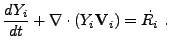
The general continuity equation for the ![]() th isotope is given in
Lagrangian formulation by
th isotope is given in
Lagrangian formulation by
The case
![]() is important for two reasons. First,
mass diffusion is often unimportant when compared to other transport
processes, such as thermal or viscous diffusion (i.e., large Lewis
numbers and/or small Prandtl numbers). Such a situation obtains, for
example, in the study of laminar flame fronts propagating through
the quiescent interior of a white dwarf. Second, this case permits
the decoupling of the reaction network solver from the
hydrodynamical solver through the use of operator splitting, greatly
simplifying the algorithm. This is the method used by the default
FLASH distribution. Setting
is important for two reasons. First,
mass diffusion is often unimportant when compared to other transport
processes, such as thermal or viscous diffusion (i.e., large Lewis
numbers and/or small Prandtl numbers). Such a situation obtains, for
example, in the study of laminar flame fronts propagating through
the quiescent interior of a white dwarf. Second, this case permits
the decoupling of the reaction network solver from the
hydrodynamical solver through the use of operator splitting, greatly
simplifying the algorithm. This is the method used by the default
FLASH distribution. Setting
![]() transforms
(18.4) into
transforms
(18.4) into
Because of the highly nonlinear temperature dependence of the
nuclear reaction rates and because the abundances themselves often
range over several orders of magnitude in value, the values of the
coefficients which appear in (18.6) and
(18.7) can vary quite significantly. As a result,
the nuclear reaction network equations are “stiff.” A system of
equations is stiff when the ratio of the maximum to the minimum
eigenvalue of the Jacobian matrix
![]() is large and
imaginary. This means that at least one of the isotopic abundances
changes on a much shorter timescale than another. Implicit or
semi-implicit time integration methods are generally necessary to
avoid following this short-timescale behavior, requiring the
calculation of the Jacobian matrix.
is large and
imaginary. This means that at least one of the isotopic abundances
changes on a much shorter timescale than another. Implicit or
semi-implicit time integration methods are generally necessary to
avoid following this short-timescale behavior, requiring the
calculation of the Jacobian matrix.
It is instructive at this point to look at an example of how
(18.6) and the associated Jacobian matrix are
formed. Consider the ![]() C(
C(![]() ,
,![]() )
)![]() O reaction,
which competes with the triple-
O reaction,
which competes with the triple-![]() reaction during helium
burning in stars. The rate
reaction during helium
burning in stars. The rate ![]() at which this reaction proceeds is
critical for evolutionary models of massive stars, since it
determines how much of the core is carbon and how much of the core
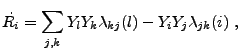
is oxygen after the initial helium fuel is exhausted. This reaction
sequence contributes to the right-hand side of (18.7) through the terms
at which this reaction proceeds is
critical for evolutionary models of massive stars, since it
determines how much of the core is carbon and how much of the core
is oxygen after the initial helium fuel is exhausted. This reaction
sequence contributes to the right-hand side of (18.7) through the terms
| (18.8) | |||
| (18.9) | |||
This release of FLASH4 contains three reaction networks.
A seven-isotope alpha-chain (Iso7) is useful for problems that
do not have enough memory to carry a larger set of isotopes.
The 13-isotope ![]() -chain plus heavy-ion reaction network (Aprox13)
is suitable for most multi-dimensional simulations of stellar phenomena,
where having a reasonably accurate energy generation rate is of primary
concern. The 19-isotope reaction network (Aprox19) has the same
-chain plus heavy-ion reaction network (Aprox13)
is suitable for most multi-dimensional simulations of stellar phenomena,
where having a reasonably accurate energy generation rate is of primary
concern. The 19-isotope reaction network (Aprox19) has the same
![]() -chain and heavy-ion reactions as the 13-isotope network, but it
includes additional isotopes to accommodate some types of hydrogen burning
(PP chains and steady-state CNO cycles), along with some aspects of
photo-disintegration into
-chain and heavy-ion reactions as the 13-isotope network, but it
includes additional isotopes to accommodate some types of hydrogen burning
(PP chains and steady-state CNO cycles), along with some aspects of
photo-disintegration into ![]() Fe. This 19 isotope reaction network
is described in Weaver, Zimmerman, & Woosley (1978).
Fe. This 19 isotope reaction network
is described in Weaver, Zimmerman, & Woosley (1978).
The networks supplied with FLASH are examples of a “hard-wired” reaction network, where each of the reaction sequences are carefully entered by hand. This approach is suitable for small networks, when minimizing the CPU time required to run the reaction network is a primary concern, although it suffers the disadvantage of inflexibility.
As mentioned in the previous section, the Jacobian matrices of nuclear reaction networks tend to be sparse, and they become more sparse as the number of isotopes increases. Since implicit or semi-implicit time integration schemes generally require solving systems of linear equations involving the Jacobian matrix, taking advantage of the sparsity can significantly reduce the CPU time required to solve the systems of linear equations.
The MA28 sparse matrix package used by FLASH is described by Duff,
Erisman, & Reid (1986). This package, which has been described
as the “Coke classic” of sparse linear algebra packages, uses a direct
- as opposed to an iterative - method for solving linear systems. Direct
methods typically divide the solution of
![]() into a symbolic LU decomposition, a numerical LU
decomposition, and a backsubstitution phase. In the symbolic LU
decomposition phase, the pivot order of a matrix is determined, and a
sequence of decomposition operations that minimizes the amount of
fill-in is recorded. Fill-in refers to zero matrix elements which
become nonzero (e.g., a sparse matrix times a sparse matrix is
generally a denser matrix). The matrix is not decomposed; only the
steps to do so are stored. Since the nonzero pattern of a chosen
nuclear reaction network does not change, the symbolic LU
decomposition is a one-time initialization cost for reaction networks.
In the numerical LU decomposition phase, a matrix with the same pivot
order and nonzero pattern as a previously factorized matrix is
numerically decomposed into its lower-upper form. This phase must be
done only once for each set of linear equations. In the
backsubstitution phase, a set of linear equations is solved with the
factors calculated from a previous numerical decomposition. The
backsubstitution phase may be performed with as many right-hand sides
as needed, and not all of the right-hand sides need to be known in
advance.
into a symbolic LU decomposition, a numerical LU
decomposition, and a backsubstitution phase. In the symbolic LU
decomposition phase, the pivot order of a matrix is determined, and a
sequence of decomposition operations that minimizes the amount of
fill-in is recorded. Fill-in refers to zero matrix elements which
become nonzero (e.g., a sparse matrix times a sparse matrix is
generally a denser matrix). The matrix is not decomposed; only the
steps to do so are stored. Since the nonzero pattern of a chosen
nuclear reaction network does not change, the symbolic LU
decomposition is a one-time initialization cost for reaction networks.
In the numerical LU decomposition phase, a matrix with the same pivot
order and nonzero pattern as a previously factorized matrix is
numerically decomposed into its lower-upper form. This phase must be
done only once for each set of linear equations. In the
backsubstitution phase, a set of linear equations is solved with the
factors calculated from a previous numerical decomposition. The
backsubstitution phase may be performed with as many right-hand sides
as needed, and not all of the right-hand sides need to be known in
advance.
MA28 uses a combination of nested dissection and frontal envelope
decomposition to minimize fill-in during the factorization stage. An
approximate degree update algorithm that is much faster
(asymptotically and in practice) than computing the exact degrees is
employed. One continuous real parameter sets the amount of searching
done to locate the pivot element. When this parameter is set to zero,
no searching is done and the diagonal element is the pivot, while when
set to unity, partial pivoting is done. Since the matrices
generated by reaction networks are usually diagonally dominant, the
routine is set in FLASH to use the diagonal as the pivot
element. Several test cases showed that using partial pivoting did not
make a significant accuracy difference but was less efficient, since
a search for an appropriate pivot element had to be performed. MA28
accepts the nonzero entries of the matrix in the
![]() ) coordinate system and typically uses 70
) coordinate system and typically uses 70![]() 90% less
storage than storing the full dense matrix.
90% less
storage than storing the full dense matrix.
GIFT is a program which generates Fortran subroutines for solving a
system of linear equations by Gaussian elimination (Gustafson,
Liniger, & Willoughby 1970; Müller 1997). The full matrix
![]() is reduced to upper triangular form, and
backsubstitution with the right-hand side b yields the solution
to
is reduced to upper triangular form, and
backsubstitution with the right-hand side b yields the solution
to
![]() . GIFT generated routines
skip all calculations with matrix elements that are zero; in this
restricted sense, GIFT generated routines are sparse, but the storage
of a full matrix is still required. It is assumed that the pivot
element is located on the diagonal and no row or column interchanges
are performed, so GIFT generated routines may become unstable if the
matrices are not diagonally dominant. These routines must decompose
the matrix for each right-hand side in a set of linear equations.
GIFT writes out (in Fortran code) the sequence of Gaussian elimination
and backsubstitution steps without any do loop constructions on the matrix
. GIFT generated routines
skip all calculations with matrix elements that are zero; in this
restricted sense, GIFT generated routines are sparse, but the storage
of a full matrix is still required. It is assumed that the pivot
element is located on the diagonal and no row or column interchanges
are performed, so GIFT generated routines may become unstable if the
matrices are not diagonally dominant. These routines must decompose
the matrix for each right-hand side in a set of linear equations.
GIFT writes out (in Fortran code) the sequence of Gaussian elimination
and backsubstitution steps without any do loop constructions on the matrix
![]() . As a result, the routines generated by GIFT can be quite
large. For the 489 isotope network discussed by Timmes (1999), GIFT
generated
. As a result, the routines generated by GIFT can be quite
large. For the 489 isotope network discussed by Timmes (1999), GIFT
generated ![]() 5.0
5.0![]() 10
10![]() lines of code! Fortunately, for
small reaction networks (less than about 30 isotopes), GIFT generated
routines are much smaller and generally faster than other linear
algebra packages.
lines of code! Fortunately, for
small reaction networks (less than about 30 isotopes), GIFT generated
routines are much smaller and generally faster than other linear
algebra packages.
The FLASH runtime parameter algebra controls which linear algebra package is used in the simulation. algebra = 1 is the default choice and invokes the sparse matrix MA28 package. algebra = 2 invokes the GIFT linear algebra routines.
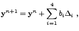
One of the time integration methods used by FLASH for evolving the
reaction networks is a 4th-order accurate Kaps-Rentrop, or Rosenbrock method. In
essence, this method is an implicit Runge-Kutta algorithm. The
reaction network is advanced over a timestep ![]() according to
according to
| (18.11) | |||
| (18.12) | |||
| (18.13) | |||
| (18.14) |
Another time integration method used by FLASH for evolving the reaction
networks is the variable order Bader-Deuflhard method (e.g., Bader &
Deuflhard 1983). The reaction network is advanced
over a large timestep ![]() from
from ![]() to
to
![]() by the
following sequence of matrix equations. First,
by the
following sequence of matrix equations. First,
| (18.16) | |||
The FLASH runtime parameter odeStepper controls which integration method is used in the simulation. The choice odeStepper = 1 is the default and invokes the variable order Bader-Deuflhard scheme. The choice odeStepper = 2 invokes the fourth order Kaps-Rentrop / Rosenbrock scheme.
For most astrophysical detonations, the shock structure is so thin that there is insufficient time for burning to take place within the shock. However, since numerical shock structures tend to be much wider than their physical counterparts, it is possible for a significant amount of burning to occur within the shock. Allowing this to happen can lead to unphysical results. The burner unit includes a multidimensional shock detection algorithm that can be used to prevent burning in shocks. If the useShockBurn parameter is set to .false., this algorithm is used to detect shocks in the Burn unit and to switch off the burning in shocked cells.
Currently, the shock detection algorithm supports Cartesian and 2-dimensional cylindrical coordinates. The basic algorithm is to compare the jump in pressure in the direction of compression (determined by looking at the velocity field) with a shock parameter (typically 1/3). If the total velocity divergence is negative and the relative pressure jump across the compression front is larger than the shock parameter, then a cell is considered to be within a shock.
This computation is done on a block by block basis. It is important that the velocity and pressure variables have up-to-date guard cells, so a guard cell call is done for the burners only if we are detecting shocks (i.e. useShockBurning = .false.).
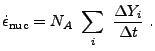
The instantaneous energy generation rate is given by the sum
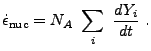 |
(18.18) |
 |
(18.19) |
The tabulation of Caughlan & Fowler (1988) is used in FLASH for most of the key nuclear reaction rates. Modern values for some of the reaction rates were taken from the reaction rate library of Hoffman (2001, priv. comm.). A user can choose between two reaction rate evaluations in FLASH. The runtime parameter useBurnTable controls which reaction rate evaluation method is used in the simulation. The choice useBurnTable = 0 is the default and evaluates the reaction rates from analytical expressions. The choice useBurnTable = 1 evaluates the reactions rates from table interpolation. The reaction rate tables are formed on-the-fly from the analytical expressions. Tests on one-dimensional detonations and hydrostatic burnings suggest that there are no major differences in the abundance levels if tables are used instead of the analytic expressions; we find less than 1% differences at the end of long timescale runs. Table interpolation is about 10 times faster than evaluating the analytic expressions, but the speedup to FLASH is more modest, a few percent at best, since reaction rate evaluation never dominates in a real production run.
Finally, nuclear reaction rate screening effects as formulated by
Wallace et al. (1982) and decreases in the energy generation rate
![]() due to neutrino losses as given by Itoh et
al. (1996) are included in FLASH.
due to neutrino losses as given by Itoh et
al. (1996) are included in FLASH.
When using explicit hydrodynamics methods, a timestep limiter must be used to ensure the stability of the numerical solution. The standard CFL limiter is always used when an explicit hydrodynamics unit is included in FLASH. This constraint does not allow any information to travel more than one computational cell per timestep. When coupling burning with the hydrodynamics, the CFL timestep may be so large compared to the burning timescales that the nuclear energy release in a cell may exceed the existing internal energy in that cell. When this happens, the two operations (hydrodynamics and nuclear burning) become decoupled.
To limit the timestep when burning is performed, an additional constraint is imposed. The limiter tries to force the energy generation from burning to be smaller than the internal energy in a cell. The runtime parameter enucDtFactor controls this ratio. The timestep limiter is calculated as
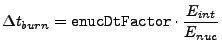 |
(18.20) |