18. Local Source Terms

Figure 18.1: The organizational structure of physics source terms, which include units such as Burn and Stir. Shaded units include only stub implementations. Only a subset of units is shown.

Figure 18.2: The organizational structure of physics source terms, with additional units, including Heatexchange.

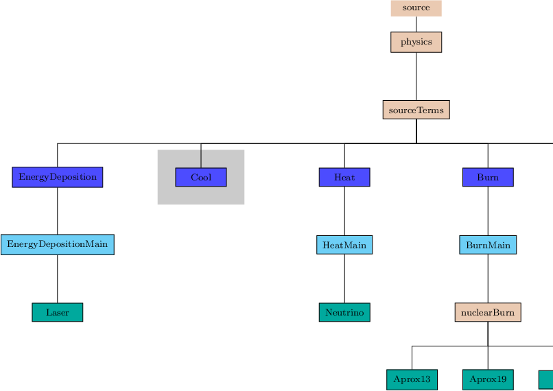
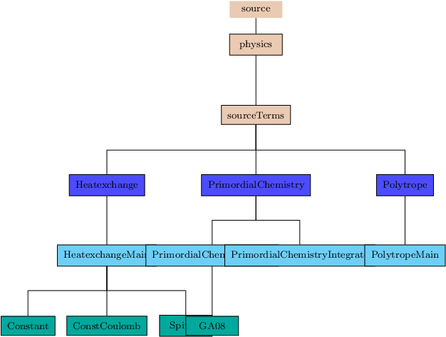
The physics/sourceTerms organizational directory contains several units that implement forcing terms. The Burn, Stir, Ionize, and Diffuse units contain implementations in FLASH4. Two other units, Cool and Heat, contain only stub level routines in their API.