18.7 Turbulence Measurement

The Turb unit implements a method to measure the local turbulence strength at the grid scale. The implementation is based on the operator $OP_2$ in Colin et al. (2000),

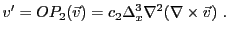$$v' = OP_2(\vec v) = c_2 \Delta_x^3\nabla^2(\nabla\times\vec v) .$$ (18.279)

Here $c_2$ is a calibration constant, set with the turb_c2 runtime variable. The default value, 0.9, was determined for the PPM hydodynamics method by Jackson et al. (2014, submitted) based on simulations of stirred turbulence. $\Delta_x$ is the grid spacing and $v$ is the velocity field on the grid. Two options are implemented for sampling the velocity field, each of which uses a 5-point stencil for the Laplacian operator. If turb_stepSize is set to 1, the stencil samples adjacent cells, if set to $2$ every other cell is sampled, for an effective stencil size of 9 points. The latter option requeres a guardcell fill between the curl and Laplacian operators. The result of equation 18.279 is stored in the TURB mesh variable.