18.3 Stir Unit

The addition of driving terms in a hydrodynamical simulation can be a useful feature, for example, in generating turbulent flows or for simulating the addition of power on larger scales (e.g., supernova feedback into the interstellar medium). The Stir unit comes in two implementations: 1) the Generate implementation, in which a divergence-free, random time-correlated `stirring' velocity is directly added at selected modes in the simulation and 2) the FromFile implementation, in which a stirring field is set up from data residing on a file. The FromFile implementation allows to set up identical stirring fields on different platforms, and thus comparisons can be made between different codes.

Before FLASH 4.2, the implementation now called Generate was the only one provided. It is still the default that is being used if one specifies just

in a Config file or -unit=physics/sourceTerms/Stir on the setup command line.

18.3.1 Stir Unit: Generate Implementation

In the generate implementation, the Stir unit directly adds a divergence-free, time-correlated `stirring' velocity at selected modes in the simulation.

The time-correlation is important for modeling realistic driving forces. Most large-scale driving forces are time-correlated, rather than white-noise; for instance, turbulent stirring from larger scales will be correlated on timescales related to the lifetime of an eddy on the scale of the simulation domain. This time correlation will lead to coherent structures in the simulation that will be absent with white-noise driving.

For each mode at each timestep, six separate phases (real and imaginary in each of the three spatial dimensions) are evolved by an Ornstein-Uhlenbeck (OU) random process (Uhlenbeck 1930). The OU process is a zero-mean, constant-rms process, which at each step `decays' the previous value by an exponential $f = e^{(\frac{\Delta t}{\tau})}$ and then adds a Gaussian random variable with a given variance, weighted by a 'driving' factor $\sqrt (1 - f^2)$. Since the OU process represents a velocity, the variance is chosen to be the square root of the specific energy input rate (set by the runtime parameter st_energy) divided by the decay time $\tau$ (st_decay). In the limit that the timestep $\Delta t \rightarrow 0$, it is easily seen that the algorithm represents a linearly-weighted summation of the old state with the new Gaussian random variable.

By evolving the phases of the stirring modes in Fourier space, imposing a divergence-free condition is relatively straightforward. At each timestep, the solenoidal component of the velocities is projected out, leaving only the non-compressional modes to add to the velocities.

The velocities are then converted to physical space by a direct Fourier transform - i.e., adding the $\sin$ and $\cos$ terms explicitly. Since most drivings involve a fairly small number of modes, this is more efficient than an FFT, since the FFT would need large numbers of modes (equal to six times the number of cells in the domain), the vast majority of which would have zero amplitude.

18.3.2 Stir Unit: FromFile Implementation

In the from file implementation, the Stir unit sets up a stirring field from data residing on a file. Here we summarize the method for driving turbulence used in Federrath et al. (2010, A&A, 512, A81). Please refer to that paper for further details.

Turbulence decays in about a crossing time, because the kinetic energy carried by the turbulence dissipates on small scales and turns into heat. In order to study the statistics of turbulence (e.g., the PDF, power spectrum, structure functions, etc.) over a significant time period thus requires continuous stirring (also called driving or forcing) with a turbulent acceleration field, which we call $\vec{f}(\vec{x},t)$ in the following.

The stirring field $\vec{f}$ is often modeled with a spatially static pattern for which the amplitude is adjusted in time. This results in a roughly constant energy input on large scales, but has the disadvantage that the turbulence is not really random, because the large-scale pattern is fixed, which may introduce undesirable systematics. Other studies model $\vec{f}$ such that it can vary in time and space to achieve a smoothly varying pattern that resembles the flow of kinetic energy from scales larger than the simulation box scale. The most widely used method to achieve this is the Ornstein-Uhlenbeck (OU) process. The OU process is a well-defined stochastic process with a finite autocorrelation timescale. It can be used to excite turbulent motions in 3D, 2D, or 1D simulations as explained in Eswaran & Pope (1988, Computers & Fluids, 16, 257).

The OU process is a stochastic differential equation describing the evolution of $\widehat{\vec{f}}$ in Fourier space ($k$-space):

$$\mathrm{d}\widehat{\vec{f}} (\vec{k},t) = f_{0 }(\vec{k})\;\mat... ...athcal{\vec{W}}(t) - \widehat{\vec{f}} (\vec{k},t) \frac{\mathrm{d}t}{T}\;.$$ (18.27)

The first term on the right hand side is a diffusion term. This term is modeled by a Wiener process $\mathcal{\vec{W}}(t)$, which adds a Gaussian random increment to the vector field given in the previous time step $\mathrm{d}t$. Wiener processes are random processes, such that

$$\mathcal{\vec{W}}(t)-\mathcal{\vec{W}}(t-\mathrm{d}t)=\mathcal{\vec{N}}(0,\mathrm{d}t)\;,$$ (18.28)

where $\mathcal{\vec{N}}(0,\mathrm{d}t)$ denotes the 3D, 2D, or 1D version of a Gaussian distribution with zero mean and standard deviation $\mathrm{d}t$. This is combined with a projection using the projection tensor $\mathcal{\underline{P}}^{ \zeta}(\vec{k})$ in Fourier space. In index notation, the projection operator reads

$$\mathcal{P}_{ij}^\zeta (\vec{k}) = \zeta \mathcal{P}_{ij}^\perp... ...l (\vec{k}) = \zeta \delta_{ij}+(1-2\zeta) \frac{k_i k_j}{\vert k\vert^2}\;,$$ (18.29)

where $\delta_{ij}$ is the Kronecker symbol, and $\mathcal{P}_{ij}^\perp = \delta_{ij} - k_i k_j / k^2$ and $\mathcal{P}_{ij}^\parallel = k_i k_j / k^2$ are the solenoidal (divergence-free) and the compressive (curl-free) projection operators, respectively. The projection operator serves to construct a purely solenoidal stirring field by setting $\zeta =1$. For $\zeta =0$, a purely compressive stirring field is obtained. Any combination of solenoidal and compressive modes can be constructed by choosing $\zeta\in[0,1]$. By changing the parameter $\zeta$, we can thus set the power of compressive modes with respect to the total power in the driving field. The analytical ratio of compressive power to total power can be derived from equation (18.29) by evaluating the norm of the compressive component of the projection tensor,

$$\left\vert(1-\zeta) \mathcal{P}_{ij}^\parallel\right\vert^2 = (1-\zeta)^2\;,$$ (18.30)

and by evaluating the norm of the full projection tensor

$$\left\vert\mathcal{P}_{ij}^\zeta\right\vert^2 = 1-2\zeta+D\zeta^2\;.$$ (18.31)

The result of the last equation depends on the dimensionality $D=1,2,3$ of the simulation, because the norm of the Kronecker symbol $\vert\delta_{ij}\vert=1, 2$ or 3 in one, two or three dimensions, respectively. The ratio of equations (18.30) and (18.31) gives the relative power in compressive modes, $F_\mathrm{long}/F_\mathrm{tot}$, as a function of $\zeta$:

$$\frac{F_\mathrm{long}}{F_\mathrm{tot}} = \frac{(1-\zeta)^2}{1-2\zeta+D\zeta^2}\;.$$ (18.32)

Figure 18.3 provides a graphical representation of this ratio for the 1D, 2D, and 3D case. For comparison, we plot numerical values of the forcing ratio obtained in eleven 3D and 2D hydrodynamical simulations by Federrath et al. (2010, A&A, 512, A81), in which we varied the forcing parameter $\zeta$ from purely compressive stirring ($\zeta =0$) to purely solenoidal stirring ($\zeta =1$) in the range $\zeta =[0,1]$, separated by $\Delta \zeta =0.1$. Note that a natural mixture of stirring modes is obtained for $\zeta=0.5$, which leads to $F_\mathrm{long}/F_\mathrm{tot}=1/3$ for 3D turbulence, and $F_\mathrm{long}/F_\mathrm{tot}=1/2$ for 2D turbulence. A simple way to understand this natural ratio is to consider longitudinal and transverse waves. In 3D, the longitudinal waves occupy one of the three spatial dimensions, while the transverse waves occupy two of the three on average. Thus, the longitudinal (compressive) part has a relative power of 1/3, while the transverse (solenoidal) part has a relative power of 2/3 in 3D. In 2D, the natural ratio is 1/2, because longitudinal and transverse waves are evenly distributed in two dimensions.

Figure 18.3: Ratio of compressive to total power of the turbulent stirring field, reprinted from Federrath et al. (2010, A&A, 512, A81) with permission by Astronomy & Astrophysics. The solid lines labelled with 1D, 2D, and 3D show the analytical expectation for this ratio, equation (18.32), as a function of the stirring parameter $\zeta$ for one-, two- and three-dimensional driving, respectively. The diamonds and squares show results of numerical simulations in 3D and 2D with $\zeta =[0,1]$, separated by $\Delta \zeta =0.1$. The two limiting cases of purely solenoidal stirring ($\zeta =1$) and purely compressive stirring ($\zeta =0$) are indicated as ”sol” and ”comp”, respectively. Note that in any 1D model, all power is in the compressive component, and thus $F_\mathrm{long}/F_\mathrm{tot}=1$, independent of $\zeta$.

The second term on the right-hand side of equation (18.27) is a drift term describing the exponential decay of the autocorrelation of $\vec{f}$. The usual procedure is to set the autocorrelation timescale equal to the turbulent crossing time, $T=L_\mathrm{peak}/V$, on the scale of energy injection, $L_\mathrm{peak}$. This type of stirring models the kinetic energy input from large-scale turbulent fluctuations breaking up into smaller and smaller structures.

The runtime parameters associated with the StirFromFile unit are described in the 18.3.3 section.

18.3.3 Using the StirFromFile Unit

18.3.3.1 Runtime Parameters

Table 18.2: Runtime parameters for the stirring module.

Variable	Type	Default	Description
useStir	boolean	.true.	switch stirring on/off
st_computeDt	boolean	.false.	restrict timestep based on stirring
st_infilename	string	"forcingfile.dat"	file containing the stirring time sequence

Table 18.2 lists the runtime parameters for the StirFromFile unit. This includes a switch for turning the stirring module on/off and a switch to restrict the timestep based on the acceleration field used for stirring (st_computeDt is switched off by default, because it is normally sufficient to restrict the timestep based on the gas velocity). Finally, st_infilename is the name of the input file containing the time and mode sequence used for stirring. This file must be prepared in advance with a separate Fortran program located in SimulationMain/StirFromFile/forcing_generator/. The reason for this structural splitting is to predetermine what the code is going to do. For instance, by preparing the time sequence of the stirring in advance, one can always reproduce exactly the full evolution of all driving patterns applied during a simulation. It also has the advantage that exactly identical stirring patterns can be applied in completely different codes, because they read the time and mode sequence from the same stirring file (Price & Federrath, 2010, MNRAS, 406, 1659).

The stirring module is compatible with any hydro or MHD solver and any grid implementation (uniform or AMR). Upon inclusion in a FLASH setup or module, the StirFromFile module defines three additional grid scalar fields, accx, accy, and accz, holding the three vector components of the stirring field $\vec{f}$.

18.3.3.2 Preparing the Stirring Sequence (st_infilename)

Table 18.3: Parameters in forcing_generator.F90 to prepare a stirring sequence.

Variable	Type	Default	Description
ndim	integer	$3$	The dimensionality of the simulation (1, 2, or 3)
xmin, xmax	real	$-0.5, 0.5$	Domain boundary coordinates in $x$ direction
ymin, ymax	real	$-0.5, 0.5$	Domain boundary coordinates in $y$ direction
zmin, zmax	real	$-0.5, 0.5$	Domain boundary coordinates in $z$ direction
st_spectform	integer	$1$	Spectral shape (0: band, 1: paraboloid)
st_decay	real	$0.5$	Autocorrelation time of the OU process, $T=L_\mathrm{peak}/V$
st_energy	real	2e-3	Determines the driving amplitude
st_stirmin	real	$6.283$	Minimum wavenumber stirred (e.g., $k_\mathrm{min}\lesssim2\pi/L_\mathrm{box}$)
st_stirmax	real	$18.95$	Maximum wavenumber stirred (e.g., $k_\mathrm{max}\gtrsim6\pi/L_\mathrm{box}$)
st_solweight	real	$1.0$	Mode mixture $\zeta =[0,1]$ in Eq. (18.32). Typical values are $1.0$: solenoidal; $0.0$: compressive; $0.5$: natural mixture.
st_seed	integer	$140281$	Random seed for stirring sequence
end_time	real	$5.0$	Final time in stirring sequence
nsteps	integer	$100$	Number of realizations between $t=0$ and end_time
outfilename	string	"forcingfile.dat"	Output name (input file st_infilename for FLASH)

The code requires a time sequence of stirring modes at runtime, which have to be prepared with the stand-alone Fortran program forcing_generator.F90 in SimulationMain/StirFromFile/forcing_generator/. A Makefile is provided in the same directory. This program prepares the time sequence of Fourier modes, which is then read by FLASH during runtime, to construct the physical acceleration fields used for stirring. It controls the spatial structure and the temporal correlation of the driving, its amplitude, the mode mixture, and the time separation between successive driving patterns. The user has to modify forcing_generator.F90 to construct a requested driving sequence and to tailor it to the desired physical situation to be modeled.

Table 18.3 lists all the parameters that can be adjusted in the main routine of forcing_generator.F90. Most of them are straightforward to set (ndim, xmin, xmax, ymin, ...^18.1), but others may require some explanation. For example, st_spectform determines the shape of the driving amplitude in Fourier space. Many colleagues drive a band (st_spectform=0), i.e., equal power injected between wavenumber modes $k_\mathrm{min}={\tt st\_stirmin}$ and $k_\mathrm{max}={\tt st\_stirmax}$. This produces a sharp transition between stirred modes and modes that are not stirred. Here we set the default to a smooth function, a paraboloid (st_spectform=1), such that most power is injected on wavenumber $k_\mathrm{peak}=(k_\mathrm{min}+k_\mathrm{max})/2$ and falls off quadratically towards both wavenumber ends, normalized such that the injected power at $k_\mathrm{min}$ and $k_\mathrm{max}$ vanishes. This has the advantage of defining a characteristic peak injection scale $k_\mathrm{peak}$ and achieves a smooth transition between stirred and non-stirred wavenumbers.

st_decay and st_energy determine the autocorrelation time of the OU process and the total injected energy, which is simply a measure for the normalization of the acceleration field. These parameters must be adjusted according to the physical setup. For instance, for a given target velocity dispersion $V$ on the injection scale $L_\mathrm{peak}=2\pi/k_\mathrm{peak}$, the autocorrelation time should be set equal to the turbulent crossing time, $T=L_\mathrm{peak}/V$. In contrast, setting st_decay to a very small or a very large number results in white noise driving or in a static driving pattern, respectively.

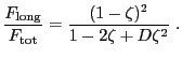
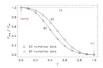
The parameter st_solweight determines whether the acceleration field will be solenoidal (divergence-free) or compressive (curl-free) or any mixture, according to Equation (18.32). Incompressible gases should naturally be driven with a purely solenoidal field ($\zeta =1$), while compressible turbulence in the interstellar medium may be driven primarily by a mixture of solenoidal and compressive modes. A detailed study of the influence of $\zeta$ is presented in Federrath et al. (2010, A&A, 512, A81).

st_seed is the random seed for the OU sequence and determines the pseudo random number sequence for the integrated Box-Muller random number generator.

Finally, end_time and nsteps determine the final physical time for stirring and the number of driving patterns to be prepared within the time period from $t=0$ to $t={\tt end\_time}$. This sets the number of equally-spaced times at which FLASH is going to read a new stirring pattern from the file. This allows the user to control how frequently a new driving pattern is constructed. A useful time separation of successive driving patterns is about 10% of a crossing time (or autocorrelation time), i.e., setting ${\tt nsteps}=10\times{\tt end\_time}/{\tt st\_decay}$. This will sample the smooth changes in the OU driving sequence sufficiently well for most applications.

18.3.4 Stirring Unit Test

An example setup using the StirFromFile unit is located in SimulationMain/StirFromFile/. The unit test can be invoked by

./setup StirFromFile -auto -3d -nxb=16 -nyb=16 -nzb=16 +ug -with-unit=physics/Hydro.

The FLASH executable must be copied into the run directory together with the standard flash.par for this setup, and together with the default forcing file (to be constructed using the standard parameters; see section 18.3.3.2). During runtime the code writes a file with the time evolution of spatially integrated quantities, amongst others, the rms Mach number and vorticity, which can used as basic code checks.