Next: 18.6 Flame Up: 18. Local Source Terms Previous: 18.4 Energy Deposition Unit Contents Index
The Heatexchange unit implements coupling among the different components (Ion, Electron, Radiation) as a simple relaxation law.
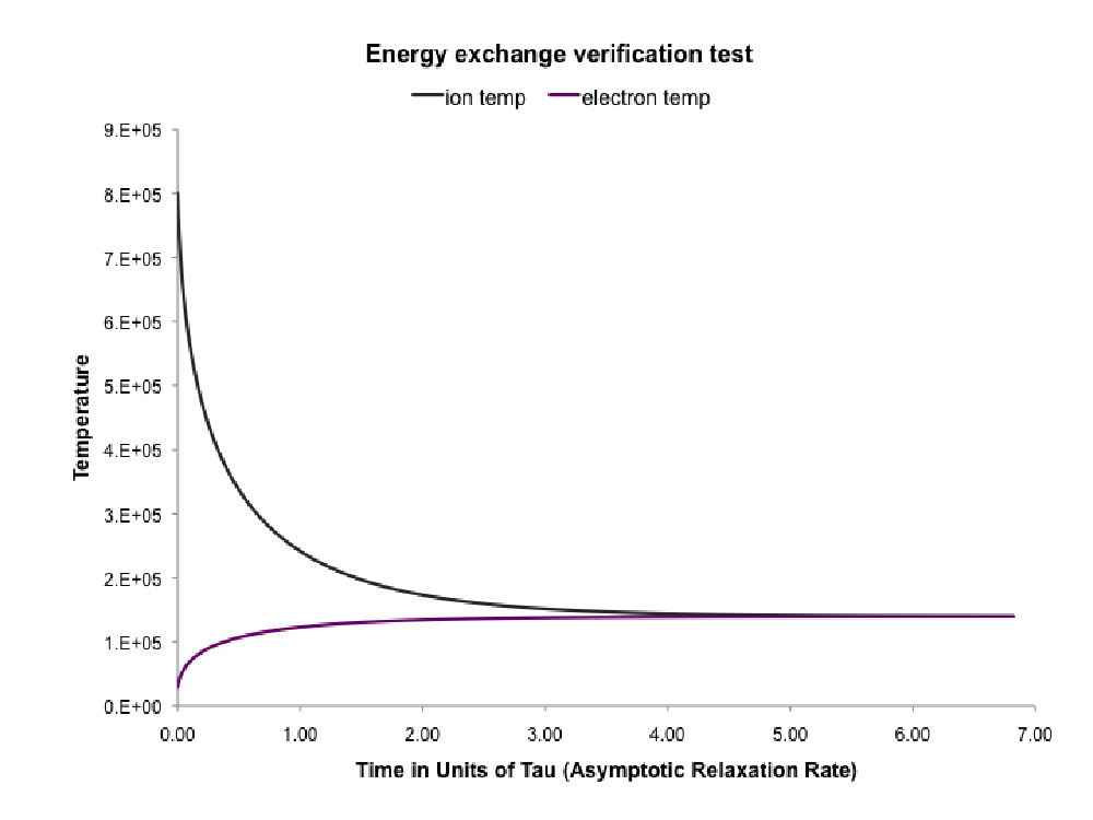
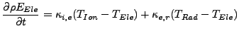
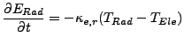
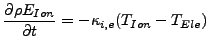
This unit is required because FLASH operator splits the electron-ion equilibration term from the rest of the calculations. All realistic 3T HEDP simulations should include the Heatexchange unit since it is responsible for equilibrating the ion/electron temperatures over time. The radiation terms in (Eqn:energyexchange) are only included when the legacy gray radiation diffusion unit is used. The more sophisticated multigroup radiation diffusion unit, described in chp:RadTrans, includes the emission and absorption internally.
There are several different implementations residing under Heatexchange unit,
The Constant and ConstCoulomb implementations are really designed to be used for testing purposes. The Spitzer and LeeMore implementation should be used for simulations of actual HEDP experiments since it is more accurate and physically realistic. This is described in detail in Sec:HeatexchangeSpitzer and Sec:HeatexchangeLeeMore.
hx_relTol runtime parameter affects the time step computed by
Heatexchange_computeDt. Basically, if the max (abs) temperature
adjustment that would be introduced in any nonzero component in any
cell is less than hx_relTol, then the time step limit is relaxed. Set
to a negative value to inherite the value of runtime parameter
eos_tolerance.
Usage: To use any implementation of Heatexchange unit, a
simulation should include the Heatexchange using an option like
-with-unit=physics/sourceTerms/Heatexchange/HeatexchangeMain/ConstCoulomb
on the setup line, or add
REQUIRES
physics/sourceTerms/Heatexchange/HeatexchangeMain/ConstCoulomb in
the Config file. The same process can be repeated for other
implementations.Constant implementation is
set as the default.
|
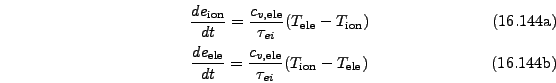
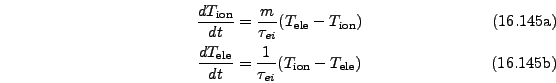
The Spitzer implementation described here and LeeMore implementation described later in Sec:HeatexchangeLeeMore should be used to model electron-ion equilibration in realistic HEDP simulations. See Sec:LaserSlab for an example of how to use the Spizter Heatexchange implementation in an HEDP simulation. Note, that this implementation only models electron-ion equilibration, and does not include any radiation related physics. In that sense it is designed to be used in conjunction with the multigroup radiation unit described in diffusion chp:RadTrans, since this unit includes the emission and absorption terms internally. Thus the equations solved by the Spitzer implementation are:
 |
 |
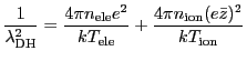
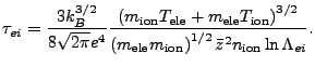
The subroutine PlasmaState_ieEquilTime is responsible for computing the
electron-ion equilibration time, ![]() . Currently, the formula
used is consistent with that given in (Atzeni, 2004) and the NRL Plasma
Formulary (Huba, 2011). The value of
. Currently, the formula
used is consistent with that given in (Atzeni, 2004) and the NRL Plasma
Formulary (Huba, 2011). The value of ![]() is shown in
(Eqn:HxSpitzerIeTime).
is shown in
(Eqn:HxSpitzerIeTime).
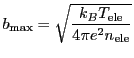
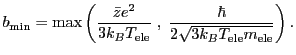
The Coulomb logarithm is the logarithmic ratio of the maximum impact parameter,
![]() , to minimum impact
parameter,
, to minimum impact
parameter,
![]() , for electron-ion collisions, i.e.,
, for electron-ion collisions, i.e.,
 |
(18.272) |
Note that in HED plasmas, there are situations where
![]() resulting in a very small or negative value.
Therefore, the Coulomb logarithm is forced to be greater than or equal to 1.0 by default (as in Brysk, 1974).
This floor value can be changed by setting the runtime parameter logLambdaFloor.
resulting in a very small or negative value.
Therefore, the Coulomb logarithm is forced to be greater than or equal to 1.0 by default (as in Brysk, 1974).
This floor value can be changed by setting the runtime parameter logLambdaFloor.
Finally, note that the runtime parameter hx_ieTimeCoef
multiplies ![]() and can be used to scale
and can be used to scale ![]() .
.
The LeeMore heat exchange uses (Eqn:HxSpitzerIeTime), but with a different expression for the Coulomb logarithm,
![]() . The expression for
. The expression for
![]() comes from Sec. III.B. of Lee & More 1984,
comes from Sec. III.B. of Lee & More 1984,
 |
(18.275) |
Like the Spitzer heat exchange model, the Coulomb logarithm in the LeeMore heat exchange is forced to be greater or equal to logLambdaFloor. Lee & More 1984 cite numerical results that conclude that the floor on the Columb logarithm should be 2.0 (instead of 1.0 as in the Spitzer heat exchange model).
It should be reiterated that the LeeMore heat exchange model just described only differs from the Spitzer heat exchange in the calculation of the Coulomb logarithm. The expression in Lee & More 1984 for the electron relaxation time (their Eq. 24) also contains Fermi-Dirac factors that we neglect here for simplicity. These factors may be incorporated into the LeeMore heat exchange model at a later date. Regardless, the LeeMore heat exchange module should be more accurate than the Spitzer heat exchange because of the improvement to the Coulomb logarithm.
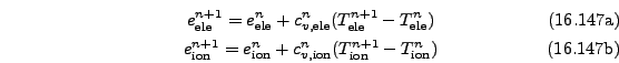
![\begin{subequations}\begin{gather}T_\mathrm{ion}^{n+1} = \left( \frac{T_\mathrm{...
... \left[ -(1+m) \frac{\Delta t}{\tau_{ei}} \right] \end{gather}\end{subequations}](img1935.png)
![$\displaystyle \ln \Lambda_{ei} = \ln \left[1 + (\frac{b_{\mathrm{max}}}{b_{\mathrm{min}}} \right]$](img1945.png)
![$\displaystyle \ln \Lambda_{ei} = \frac{1}{2} \ln \left[ 1 + \left( \frac{b_{\mathrm{max}}}{b_{\mathrm{min}}} \right)^2 \right]$](img1951.png)