35.5 Burn Test Problem

The Cellular Nuclear Burning problem is used primarily to test the function of the Burn simulation unit. The problem exhibits regular steady-state behavior and is based on one-dimensional models described by Chappman (1899) and Jouguet (1905) and Zel'dovich (Ostriker 1992), von Neumann (1942), and Doring (1943). This problem is solved in two dimensions. A complete description of the problem can be found in a recent paper by Timmes, Zingale et al(2000).

A 13 isotope $\alpha$ -chain plus heavy-ion reaction network is used in the calculations. A definition of what we mean by an $\alpha$ -chain reaction network is prudent. A strict $\alpha$ -chain reaction network is only composed of ( $\alpha$ , $\gamma$ ) and ( $\gamma$ , $\alpha$ ) links among the 13 isotopes He, $^{12}$ C, $^{16}$ O, $^{20}$ Ne, $^{24}$ Mg, $^{28}$ Si, $^{32}$ S, $^{36}$ Ar, $^{40}$ Ca, $^{44}$ Ti, $^{48}$ Cr, $^{52}$ Fe, and $^{56}$ Ni. It is essential, however, to include ( $\alpha$ ,p)(p, $\gamma$ ) and ( $\gamma$ ,p)(p, $\alpha$ ) links in order to obtain reasonably accurate energy generation rates and abundance levels when the temperature exceeds $\sim$ 2.5 $\times$ 10 $^{9}$ K. At these elevated temperatures the flows through the ( $\alpha$ ,p)(p, $\gamma$ ) sequences are faster than the flows through the ( $\alpha$ , $\gamma$ ) channels. An ( $\alpha$ ,p)(p, $\gamma$ ) sequence is, effectively, an ( $\alpha$ , $\gamma$ ) reaction through an intermediate isotope. In our $\alpha$ -chain reaction network, we include 8 ( $\alpha$ ,p)(p, $\gamma$ ) sequences plus the corresponding inverse sequences through the intermediate isotopes $^{27}$ Al, $^{31}$ P, $^{35}$ Cl, $^{39}$ K, $^{43}$ Sc, $^{47}$ V, $^{51}$ Mn, and $^{55}$ Co by assuming steady state proton flows. The two-dimensional calculations are performed in a planar geometry of size 256.0 cm by 25.0 cm. The initial conditions consist of a constant density of 10 g cm $^{-3}$ , temperature of 2 $\times$ 10 $^{8}$ K, composition of pure carbon X( $^{12}$ C)=1, and material velocity of $v_{x}=v_{y}$ = 0 cm s $^{-1}$ . Near the x=0 boundary the initial conditions are perturbed to the values given by the appropriate Chapman-Jouguet solution: a density of 4.236 $\times$ 10 g cm $^{-3}$ , temperature of 4.423 $\times$ 10 K, and material velocity of $v_{x}$ = 2.876 $\times$ 10 cm s $^{-1}$ . Choosing different values or different extents of the perturbation simply change how long it takes for the initial conditions to achieve a near ZND state, as well as the block structure of the mesh. Each block contains 8 grid points in the x-direction, and 8 grid points in the y-direction. The default parameters for cellular burning are given in Table 35.16.

**Table 35.16:** Runtime parameters used with the `Cellular` test problem.
Variable	Type	Default	Description
`xhe4`	real	0.0	Initial mass fraction of He4
`xc12`	real	1.0	Initial mass fraction of C12
`xo16`	real	0.0	Initial mass fraction of O16
`rhoAmbient`	real	1 $\times$ 10 $^{7}$	Density of cold upstream material.
`tempAmbient`	real	2 $\times$ 10 $^{8}$	Temperature of cold upstream material.
`velxAmbient`	real	0.0	X-velocity of cold upstream material.
`rhoPerturb`	real	4.236 $\times$ 10 $^{7}$	Density of the post shock material.
`tempPerturb`	real	4.423 $\times$ 10 $^{9}$	Temperature of the post shock material.
`velxPerturb`	real	2.876 $\times$ 10 $^{8}$	X-velocity of the post shock material.
`radiusPerturb`	real	25.6	Distance below which the perturbation is applied.
`xCenterPerturb`	real	0.0	X-position of the origin of the perturbation
`yCenterPerturb`	real	0.0	Y-position of the origin of the perturbation
`zCenterPerturb`	real	0.0	Z-position of the origin of the perturbation
`usePseudo1d`	logical	`.false.`	Defaults to a spherical configuration. Set to `.true.` if you want to use a 1d configuration, that is copied in the y and z directions.
`noiseAmplitude`	real	1.0 $\times$ 10 $^{-2}$	Amplitude of the white noise added to the perturbation.
`noiseDistance`	real	5.0	The distance above the starting radius to which white noise is added.

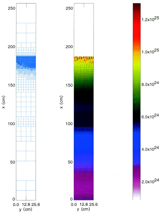
The initial conditions and perturbation given above ignite the nuclear fuel, accelerate the material, and produce an over-driven detonation that propagates along the x-axis. The initially over-driven detonation is damped to a near ZND state on short time-scale. 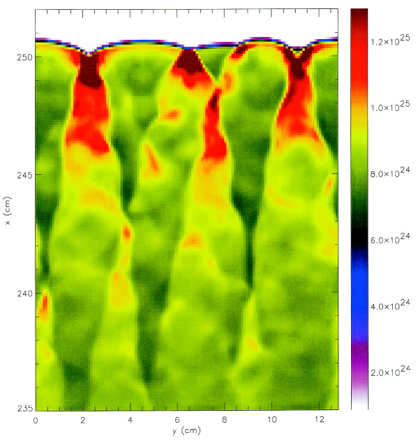After some time, which depends on the spatial resolution and boundary conditions, longitudinal instabilities in the density cause the planar detonation to evolve into a complex, time-dependent structure. Figure 35.70 shows the pressure field of the detonation after 1.26 $\times$ 10 $^{-7}$ s. The interacting transverse wave structures are particularly vivid, and extend about 25 cm behind the shock front. Figure 35.71 shows a close up of this traverse wave region. Periodic boundary conditions are used at the walls parallel to the y-axis while reflecting boundary conditions were used for the walls parallel to the x-axis.

35.5 Burn Test Problem

35.5.1 Cellular Nuclear Burning