35.4 Particles Test Problems

These problems are primarily designed to test the functioning of the particle tracking routines within FLASH4.

35.4.1 Two-particle Orbit

The Orbit problem tests the mapping of particle positions to gridded density fields, the mapping of gridded potentials onto particle positions to obtain particle forces, and the time integration of particle motion. The initial conditions consist of two particles of unit mass and separation $r_0$ located at positions $(x,y,z) = (0.5(L_x\pm r_0),0.5L_y,0.5L_z)$, where $(L_x,L_y,L_z)$ are the dimensions of the computational volume. The initial particle velocity vectors are parallel to the $y$-axis and have magnitude

$$\vert v\vert = \sqrt{2GM\over r_0} ,$$ (35.47)

if a constant gravitational field due to a point mass $M$ at $(0.5L_x,0.5L_y,0.5L_z)$ is employed, or

$$\vert v\vert = {1\over2}\sqrt{2G\over r_0} ,$$ (35.48)

if the particles are self-gravitating. The correct behavior is for the particles to orbit the center of the grid in a circle with constant velocity. Figure 35.67 shows a typical pair of particle trajectories for this problem

Figure 35.67: Particle trajectories in the Orbit test problem for a 3D grid at a fixed refinement level of 2. There is no motion along the z-axis.

No specific gravity unit is required by the problem configuration file, because the problem is intended to be run with either a fixed external field or the particles' own field. If the particles are to orbit in an external field (ext_field = .true.), the field is assumed to be a central point-mass field (physics/Gravity/GravityMain/PointMass), and the parameters for that unit should be assigned appropriate values. If the particles are self-gravitating (ext_field = .false.), the physics/Gravity/GravityMain/Poisson unit should be included in the code, and a Poisson solver that supports isolated boundary conditions should be used (grav_boundary_type = "isolated").

In either case, long-range forces for the particles must be turned on, or else they will not experience any accelerations at all. This can be done using the particle-mesh method by including the unit Particles/ParticlesMain/active/longRange/gravity/ParticleMesh.

FLASH3 Transition: Although the Multipole solver can work with the Orbit problem, the solutions are very poor. We strongly recommend the use of Multigrid solver with this problem.

As of FLASH 2.1 both the multigrid and multipole solvers support isolated boundary conditions. This problem should be run in three dimensions.

Grid interpolation: The FLASH2 user guide recommends that this problem be run with conservative, quadratic interpolants (such as mesh/amr/paramesh2.0/quadratic_cartesian) and monotonicity enforcement turned off (monotone = .false.). In FLASH4, you should use the default 2nd order monotonic interpolation scheme (see Sec:gridinterp) in PARAMESH 4.

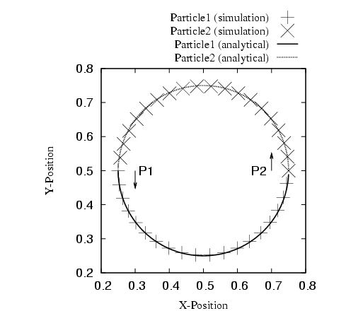
The two-particle orbit problem uses the runtime parameters listed in Table 35.13 in addition to the regular ones supplied with the code.

Table 35.13: Runtime parameters used in the orbit test problem.

Variable	Type	Default	Description
separation	real	0.5	Initial particle separation ($r_0$)
ext_field	logical	.false.	Whether to make the particles self-gravitating or to have them orbit in an external potential. In the former case GravityMain/Poisson should be used; in the latter, GravityMain/PointMass.

35.4.2 Zel'dovich Pancake

The cosmological pancake problem (Zel'dovich 1970), Pancake, provides a good simultaneous test of the hydrodynamics, particle dynamics, Poisson solver, and cosmological expansion modules. Analytic solutions well into the nonlinear regime are available for both $N$-body and hydrodynamical codes (Anninos & Norman 1994), permitting an assessment of the code's accuracy. After caustic formation the problem provides a stringent test of the code's ability to track thin, poorly resolved features and strong shocks using most of the basic physics needed for cosmological problems. Also, as pancakes represent single-mode density perturbations, coding this test problem is useful as a basis for creating more complex cosmological initial conditions.

We set the initial conditions for the pancake problem in the linear regime using the analytic solution given by Anninos and Norman (1994). In a universe with $\Omega_0=1$ at redshift $z$, a perturbation of wavenumber $k$ which collapses to a caustic at redshift $z_c<z$ has comoving density and velocity given by

$$\rho(x_e;z) = \bar{\rho}\left[1 + {1+z_c\over1+z}\cos\left(kx_\ell\right) \right]^{-1}$$ (35.49)

$$v(x_e;z) = -H_0(1+z)^{1/2}(1+z_c){\sin kx_\ell\over k} ,$$ (35.50)

where $\bar{\rho}$ is the comoving mean density. Here $x_e$ is the distance of a point from the pancake midplane, and $x_\ell$ is the corresponding Lagrangian coordinate, found by iteratively solving

$$x_e = x_\ell - {1+z_c\over 1+z}{\sin kx_\ell\over k} .$$ (35.51)

The temperature solution is determined from the density under the assumption that the gas is adiabatic with ratio of specific heats $\gamma$:

$$T(x_e;z) = (1+z)^2\bar{T}_{\rm fid}\left[\left({1+z_{\rm fid}\over 1+z} \right)^3 {\rho(x_e;z_{\rm fid})\over\rho(x_e;z)}\right]^{\gamma-1} .$$ (35.52)

The mean temperature $\bar{T}_{\rm fid}$ is specified at a redshift $z_{\rm fid}$.

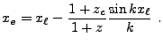
Dark matter particles are initialized using the same solution as the gas. The Lagrangian coordinates $x_\ell$ are assigned to lie on a uniform grid. The corresponding perturbed coordinates $x_e$ are computed using (35.51). Particle velocities are assigned using (35.50).

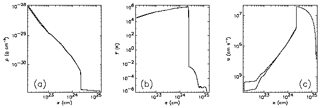
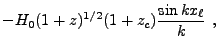
At caustic formation ($z=z_c$), planar shock waves form in the gas on either side of the pancake midplane and begin to propagate outward. A small region at the midplane is left unshocked. Immediately behind the shocks, the comoving density and temperature vary approximately as

$$\rho(x_e;z) \approx \bar{\rho}{18\over\left(kx_\ell\right)^2} {\left(1+z_c\right)^3\over\left(1+z\right)^3}$$ (35.53)

$$T(x_e;z) \approx {\mu H_0^2\over6k_Bk^2}\left(1+z_c\right) \left(1+z\right)^2\left(kx_\ell\right)^2 .$$

At the midplane, which undergoes adiabatic compression, the comoving density and temperature are approximately

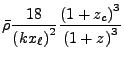
$$\rho_{\rm center} \approx \bar{\rho}\left[{1+z_{\rm fid}\over 1+z}\right]^3 \left[{3H_0^2\m... ...} {\left(1+z_c\right)^4\left(1+z\right)^3\over 1+z_{\rm fid}}\right]^{1/\gamma}$$ (35.54)

$$T_{\rm center} \approx {3H_0^2\mu\over k_Bk^2} \left(1+z\right)^2 \left(1+z_c\right)^4{\bar{\rho}\over\rho_{\rm center}} .$$

An example FLASH calculation of the post-caustic gas solution appears in Figure 35.68.

Figure: Example solution for the gas in a mixed particle/gas Zel'dovich Pancake problem. A comoving wavelength $\lambda = 10$ Mpc, caustic redshift $z_c = 5$, fiducial redshift $z_{\rm fid} = 200$, and fiducial temperature $T_{\rm fid} = 550$ K were used together with a Hubble constant of 50 km s$^{-1}$ Mpc$^{-1}$. The cosmological model was flat with a baryonic fraction of 0.15. Results are shown for redshift $z=0$. An adaptive mesh with an effective resolution of 1024 cells was used. Other parameters for this run were as described in the text. The distance $x$ is measured from the pancake midplane. (a) Gas density. (b) Gas temperature. (c) Gas velocity.

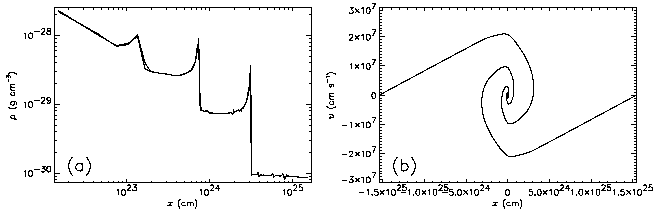
Because they are collisionless, the particles behave very differently than the gas. As particles accelerate toward the midplane, their phase profile develops a backwards “S” shape. At caustic formation the velocity becomes multivalued at the midplane. The region containing multiple streams grows in size as particles pass through the midplane. At the edges of this region (the caustics, or the inflection points of the “S”), the particle density is formally infinite, although the finite force resolution of the particles keeps the height of these peaks finite. Some of the particles that have passed through the midplane fall back and form another pair of caustics, twisting the phase profile again. Because each of these secondary caustics contains five streams of particles rather than three, the second pair of density peaks are higher than the first pair. This caustic formation process repeats arbitrarily many times in the analytic solution. In practice, the finite number of particles and the finite force resolution limit the number of caustics that are observed. An example FLASH calculation of the post-caustic particle solution appears in Figure 35.69.

Figure 35.69: Example solution for the dark matter in a mixed particle/gas Zel'dovich pancake. Perturbation and cosmological parameters were the same as in Figure 35.68. Results are shown for redshift $z=0$. An adaptive mesh with an effective resolution of 1024 cells was used. The number of particles used was 8192. Other parameters for this run were as described in the text. Distance $x$ is measured from the pancake midplane. (a) Dark matter density. (b) Dark matter phase diagram showing particle positions $x$ and velocities $v$.

The 2D pancake problem in FLASH4 uses the runtime parameters listed in Table 35.14 in addition to the regular ones supplied with the code.

This problem uses periodic boundary conditions and is intrinsically one-dimensional, but it can be run using Cartesian coordinates in 1D, 2D, or 3D, with the pancake midplane tilted with respect to the coordinate axes if desired.

Table 35.14: Runtime parameters used with the 2D pancake test problem.

Variable	Type	Default	Description
lambda	real	3.0857 $\times10^{25}$	Wavelength of the initial perturbation ($2\pi/k$)
zcaustic	real	5.	Redshift at which pancake forms a caustic ($z_c$)
Tfiducial	real	550.	Fiducial gas temperature ( $T_{\rm fid}$)
zfiducial	real	200.	Redshift at which gas temperature is $T_{\rm fid}$ ( $z_{\rm fid}$)
xangle	real	0.	Angle made by pancake normal with the $x$-axis (degrees)
yangle	real	90.	Angle made by pancake normal with the $y$-axis (degrees)
pt_numX	integer	128	Number of particles along $x$-side of initial particle “grid”
pt_numY	integer	128	Number of particles along $y$-side of initial particle “grid”
pt_numZ	integer	1	Number of particles along $z$-side of initial particle “grid”

35.4.3 Modified Huang-Greengard Poisson Test

The PoisParticles problem is designed to generate a refined grid from the distribution of particles in the computational domain. In other words, create a grid which is more refined in places where there is a clustering of particles. It is a modified form of the PoisTest simulation described in Sec:SimulationPoisTest. Recall that the PoisTest problem involves the creation of a highly refined grid, which is used to test grid refinement.

In the PoisParticles problem, the density stored in the grid is used as an indicator of where to create new particles. Here, the number of particles created in each region of the grid is proportional to the grid density, i.e., more particles are created in regions where there is a high density. Each new particle is assigned a mass, which is taken from the density in the grid, so that mass is conserved.

The flash.par parameters shown in Table 35.15 specify that the grid should refine until at most 5 particles exist per block. This creates a refined grid similar to the Poistest problem.

Table 35.15: Runtime parameters used with the PoisParticles test problem.

Variable	Type	Value	Description
refine_on_particle_count	logical	.true.	On/Off flag for refining the grid according to particle count.
max_particles_per_blk	integer	5	Grid refinement criterion which specifies maximum number of particles per block.