8.6 Adaptive Mesh Refinement (AMR) Grid with Paramesh

The default package in FLASH is PARAMESH (MacNeice et al. 1999) for implementing the adaptive mesh refinement (AMR) grid. PARAMESH uses a block-structured adaptive mesh refinement scheme similar to others in the literature (e.g., Parashar 1999; Berger & Oliger 1984; Berger & Colella 1989; DeZeeuw & Powell 1993). It also shares ideas with schemes which refine on an individual cell basis (Khokhlov 1997). In block-structured AMR, the fundamental data structure is a block of cells arranged in a logically Cartesian fashion. “Logically Cartesian” implies that each cell can be specified using a block identifier (processor number and local block number) and a coordinate triple $(i,j,k)$, where $i=1\ldots{\tt nxb}$, $j=1\ldots{\tt nyb}$, and $k=1\ldots{\tt nzb}$ refer to the $x$-, $y$-, and $z$-directions, respectively. It does not require a physically rectangular coordinate system; for example a spherical grid can be indexed in this same manner.

The complete computational grid consists of a collection of blocks with different physical cell sizes, which are related to each other in a hierarchical fashion using a tree data structure. The blocks at the root of the tree have the largest cells, while their children have smaller cells and are said to be refined. Three rules govern the establishment of refined child blocks in PARAMESH. First, a refined child block must be one-half as large as its parent block in each spatial dimension. Second, a block's children must be nested; i.e., the child blocks must fit within their parent block and cannot overlap one another, and the complete set of children of a block must fill its volume. Thus, in $d$ dimensions a given block has either zero or $2^d$ children. Third, blocks which share a common border may not differ from each other by more than one level of refinement.

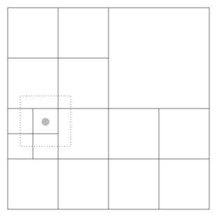
A simple two-dimensional domain is shown in Figure 8.5, illustrating the rules above. Each block contains ${\tt nxb}\times{\tt nyb}\times{\tt nzb}$ interior cells and a set of guard cells. The guard cells contain boundary information needed to update the interior cells. These can be obtained from physically neighboring blocks, externally specified boundary conditions, or both.

Figure 8.5: A simple computational domain showing varying levels of refinement in a total of 16 blocks. The dotted lines outline the guard cells for the block marked with a circle.

The number of guard cells needed depends upon the interpolation schemes and the differencing stencils used by the various physics units (usually hydrodynamics). For the explicit PPM algorithm distributed with FLASH, four guard cells are needed in each direction, as illustrated in Figure 8.4. The blocksize while using the adaptive grid is fixed at compile time, resulting in static memory allocation. The total number of blocks a processor can manage is determined by MAXBLOCKS, which can be overridden at setup time with the setup ...-maxblocks=# argument. The amount of memory consumed by the Grid data structure of code when running with PARAMESH is ${\tt NUNK\_VARS} \times (2*{\tt nguard}+{\tt nxb}) \times (2*{\tt nguard}+{\tt nyb}) \times (2*{\tt nguard}+{\tt nzb}) \times {\tt MAXBLOCKS}$. PARAMESH also needs memory to store its tree data structure for adaptive mesh management, over and above what is already mentioned with Uniform Grid. As the levels of refinement increase, the size of the tree also grows.

PARAMESH handles the filling of guard cells with information from other blocks or, at the boundaries of the physical domain, from an external boundary routine (see Sec:BndryCond). If a block's neighbor exists and has the same level of refinement, PARAMESH fills the corresponding guard cells using a direct copy from the neighbor's interior cells. If the neighbor has a different level of refinement, the data from the neighbor's cells must be adjusted by either interpolation (to a finer level of resolution) or averaging (to a coarser level)--see Sec:gridinterp below for more information. If the block and its neighbor are stored in the memory of different processors, PARAMESH handles the appropriate parallel communications (blocks are never split between processors). The filling of guard cells is a global operation that is triggered by calling Grid_fillGuardCells.

Grid Interpolation is also used when filling the blocks of children newly created in the course of automatic refinement. This happens during Grid_updateRefinement processing. Averaging is also used to regularly update the solution data in at least one level of parent blocks in the oct-tree. This ensures that after leaf nodes are removed during automatic refinement processing (in regions of the domain where the mesh is becoming coarser), the new leaf nodes automatically have valid data. This averaging happens as an initial step in Grid_fillGuardCells processing.

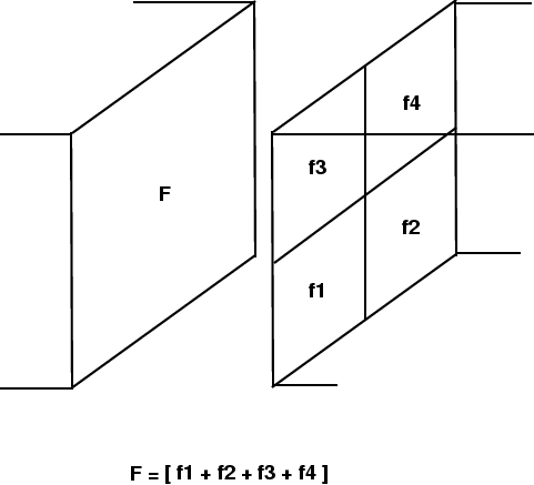
PARAMESH also enforces flux conservation at jumps in refinement, as described by Berger and Colella (1989). At jumps in refinement, the fluxes of mass, momentum, energy (total and internal), and species density in the fine cells across boundary cell faces are summed and passed to their parent. The parent's neighboring cell will be at the same level of refinement as the summed flux cell because PARAMESH limits the jumps in refinement to one level between blocks. The flux in the parent that was computed by the more accurate fine cells is taken as the correct flux through the interface and is passed to the corresponding coarse face on the neighboring block (see Figure 8.6). The summing allows a geometrical weighting to be implemented for non-Cartesian geometries, which ensures that the proper volume-corrected flux is computed.

Figure 8.6: Flux conservation at a jump in refinement. The fluxes in the fine cells are added and replace the coarse cell flux (F).

8.6.1 Additional Data Structures

PARAMESH maintains much additional information about the mesh. In particular, oct-tree related information is kept in various arrays which are declared in a F90 module called “tree”. It includes the physical coordinate of a block's center, its physical size, level of refinement, and much more. These data structures also acts as temporary storage while updating refinement in the grid and moving the blocks. This metadata should in general not be accessed directly by application code. The Grid API contains subroutines for accessing the most important pars of this metadata on a block by block basis, like Grid_getBlkBoundBox, Grid_getBlkCenterCoords, Grid_getBlkPhysicalSize, Grid_getBlkRefineLevel, and Grid_getBlkType.

FLASH has its own oneBlock data structure that stores block specific information. This data structure keeps the physical coordinates of each cell in the block. For each dimension, the coordinates are stored for the LEFT_EDGE, the RIGHT_EDGE and the center of the cell. The coordinates are determined from “cornerID” which is also a part of this data structure.

The concept of cornerID was introduced in FLASH3; it serves three purposes. First, it creates a unique global identity for every cell that can come into existence at any time in the course of the simulation. Second, it can prevent machine precision error from creeping into the spatial coordinates calculation. Finally, it can help pinpoint the location of a block within the oct-tree of PARAMESH. Another useful integer variable is the concept of a stride. A stride indicates the spacing factor between one cell and the cell directly to its right when calculating the cornerID. At the maximum refinement level, the stride is $1$, at the next higher level it is $2$, and so on. Two consecutive cells at refinement level $n$ are numbered with a stride of $2^{lrefine\_max-n}$ where $1 \le n \le lrefine\_max$.

The routine Grid_getBlkCornerID provides a convenient way for the user to retrieve the location of a block or cell. A usage example is provided in the documentation for that routine. The user should retrieve accurate physical and grid coordinates by calling the routines Grid_getBlkCornerID, Grid_getCellCoords, Grid_getBlkCenterCoords and Grid_getBlkPhysicalSize, instead of calculating their own from local block information, since they take advantage of the cornerID scheme, and therefore avoid the possibility of introducing machine precision induced numerical drift in the calculations.

8.6.2 Grid Interpolation (and Averaging)

The adaptive grid requires data interpolation or averaging when the refinement level (i.e., mesh resolution) changes in space or in time. ^8.3If during guardcell filling a block's neighbor has a coarser level of refinement, the neighbor's cells are used to interpolate guard cell values to the cells of the finer block. Interpolation is also used when filling the blocks of children newly created in the course of automatic refinement. Data averaging is used to adapt data in the opposite direction, i.e., from fine to coarse.

In the AMR context, the term prolongation is used to refer to data interpolation (because it is used when the tree of blocks grows longer). Similarly, the term restriction is used to refer to fine-to-coarse data averaging.

The algorithm used for restriction is straightforward (equal-weight) averaging in Cartesian coordinates, but has to take cell volume factors into account for curvilinear coordinates; see Sec:Non-Cart Prol/Rest.

PARAMESH supports various interpolation schemes, to which user-specified interpolation schemes can be added. FLASH4 currently allows to choose between two interpolation schemes:

1. monotonic
2. native

The choice is made at setup time, see Sec:ListSetupArgs.

The versions of PARAMESH supplied with FLASH4 supply their own default interpolation scheme, which is used when FLASH4 is configured with the -gridinterpolation=native setup option (see Sec:ListSetupArgs). The default schemes are only appropriate for Cartesian coordinates. If FLASH4 is configured with curvilinear support, an alternative scheme (appropriate for all supported geometries) is compiled in. This so-called “monotonic” interpolation attempts to ensure that interpolation does not introduce small-scale non-monotonicity in the data. The order of “monotonic” interpolation can be chosen with the interpol_order runtime parameter. See Sec:Non-Cart Prol/Rest for some more details on prolongation for curvilinear coordinates. At setup time, monotonic interpolation is the default interpolation used.

8.6.2.1 Interpolation for mass-specific solution variables

To accurately preserve the total amount of conserved quantities, the interpolation routines have to be applied to solution data in conserved, i.e., volume-specific, form. However, many variables are usually stored in the unk array in mass-specific form, e.g., specific internal and total energies, velocities, and mass fractions. See Sec:ConfigFileSyntax for how to use the optional TYPE attribute in a Config file's VARIABLE definitions to inform the Grid unit which variables are considered mass-specific.

FLASH4 provides three ways to deal with this:

1. Do nothing--i.e., assume that ignoring the difference between mass-specific and conserved form is a reasonable approximation. Depending on the smoothness of solutions in regions where refinement, derefinement, and jumps in refinement level occur, this assumption may be acceptable. This behavior can be forced by setting the convertToConsvdInMeshInterp runtime parameter to .false.

2. Convert mass-specific variables to conserved form in all blocks throughout the physical domain before invoking a Grid function that may result in some data interpolation or restriction (refinement, derefinement, guardcell filling); and convert back after these functions return. Conversion is done by cell-by-cell multiplication with the density (i.e., the value of the “dens” variable, which should be declared as  
   

   VARIABLE dens TYPE: PER_VOLUME
   

   in a Config file).

   This behavior is available in both PARAMESH 2 and PARAMESH 4. It is enabled by setting the
   convertToConsvdForMeshCalls runtime parameter and corresponds roughly to FLASH2 with
   conserved_var enabled.

3. Convert mass-specific variables to conserved form only where and when necessary, from the Grid user's point of view as part of data interpolation. Again, conversion is done by cell-by-cell multiplication with the value of density. In the actual implementation of this approach, the conversion and back-conversion operations are closely bracketing the interpolation (or restriction) calls. The implementation avoids spurious back-and-forth conversions (i.e., repeated successive multiplications and divisions of data by the density) in blocks that should not be modified by interpolation or restriction.

   This behavior is available only for PARAMESH 4. As of FLASH4, this is the default behavior whenever available. It can be enabled explicitly (only necessary in setups that change the default) by setting the
   convertToConsvdInMeshInterp runtime parameter.

8.6.3 Refinement

8.6.3.1 Refinement Criteria

The refinement criterion used by PARAMESH is adapted from Löhner (1987). Löhner's error estimator was originally developed for finite element applications and has the advantage that it uses a mostly local calculation. Furthermore, the estimator is dimensionless and can be applied with complete generality to any of the field variables of the simulation or any combination of them.

FLASH3 Transition: FLASH4 does not define any refinement variables by default. Therefore simulations using AMR have to make the appropriate runtime parameter definitions in flash.par, or in the simulation's Config file. If this is not done, the program generates a warning at startup, and no automatic refinement will be performed. The mistake of not specifying refinement variables is thus easily detected. To define a refinement variable, use refine_var_# (where # stands for a number from 1 to 4) in the flash.par file.

Löhner's estimator is a modified second derivative, normalized by the average of the gradient over one computational cell. In one dimension on a uniform mesh, it is given by

$$E_{i} = { \frac{ \mid u_{i+1} - 2u_{i} + u_{i-1} \mid} { \mid u_{... ...+ \epsilon [ \mid u_{i+1} \mid + 2 \mid u_{i} \mid + \mid u_{i-1} \mid ] } } ,$$ (8.1)

where $u_i$ is the refinement test variable's value in the $i$th cell. The last term in the denominator of this expression acts as a filter, preventing refinement of small ripples, where $\epsilon$ should be a small constant.

When extending this criterion to multidimensions, all cross derivatives are computed, and the following generalization of the above expression is used

$$E_{i_1i_2i_3} = \left\{ {\displaystyle \sum_{pq}\left({ \frac{\pa... ...over \partial x_p\partial x_q} \Delta x_p\Delta x_q \right]^2 } \right\}^{1/2},$$ (8.2)

where the sums are carried out over coordinate directions, and where, unless otherwise noted, partial derivatives are evaluated at the center of the $i_1i_2i_3$-th cell.

The estimator actually used in FLASH4's default refinement criterion is a modification of the above, as follows:

$$E_{i} = { \mid u_{i+2} - 2u_{i} + u_{i-2} \mid \over \mid u_{i+2}... ...d + \epsilon [ \mid u_{i+2} \mid + 2 \mid u_{i} \mid + \mid u_{i-2} \mid ] } ,$$ (8.3)

where again $u_i$ is the refinement test variable's value in the $i$th cell. The last term in the denominator of this expression acts as a filter, preventing refinement of small ripples, where $\epsilon$ is a small constant.

When extending this criterion to multidimensions, all cross derivatives are computed, and the following generalization of the above expression is used

$$E_{i_Xi_Yi_Z} = \left\{ {\displaystyle \sum_{pq}\left({\partial^2... ...\vert u_{pq}\right\vert}\over \Delta x_p\Delta x_q} \right]^2 } \right\}^{1/2},$$ (8.4)

where again the sums are carried out over coordinate directions, where, unless otherwise noted, partial derivatives are actually finite-difference approximations evaluated at the center of the $i_Xi_Ji_K$-th cell, and $\bar{\left\vert u_{pq}\right\vert}$ stands for an average of the values of $\left\vert u\right\vert$ over several neighboring cells in the $p$ and $q$ directions.

The constant $\epsilon$ is by default given a value of $10^{-2}$, and can be overridden through the refine_filter_# runtime parameters. Blocks are marked for refinement when the value of $E_{i_Xi_Yi_Z}$ for any of the block's cells exceeds a threshold given by the runtime parameters refine_cutoff_#, where the number # matching the number of the refine_var_# runtime parameter selecting the refinement variable. Similarly, blocks are marked for derefinement when the values of $E_{i_Xi_Yi_Z}$ for all of the block's cells lie below another threshold given by the runtime parameters derefine_cutoff_#.

Although PPM is formally second-order and its leading error terms scale as the third derivative, we have found the second derivative criterion to be very good at detecting discontinuities and sharp features in the flow variable $u$. When Particles (active or tracer) are being used in a simulation, their count in a block can also be used as a refinement criterion by setting refine_on_particle_count to true and setting max_particles_per_blk to the desired count.

8.6.3.2 Refinement Processing

Each processor decides when to refine or derefine its blocks by computing a user-defined error estimator for each block. Refinement involves creation of either zero or $2^d$ refined child blocks, while derefinement involves deletion of all of a parent's child blocks ($2^d$ blocks). As child blocks are created, they are temporarily placed at the end of the processor's block list. After the refinements and derefinements are complete, the blocks are redistributed among the processors using a work-weighted Morton space-filling curve in a manner similar to that described by Warren and Salmon (1987) for a parallel treecode. An example of a Morton curve is shown in Figure 8.7.

Figure 8.7: Morton space-filling curve for adaptive mesh grids.

During the distribution step, each block is assigned a weight which estimates the relative amount of time required to update the block. The Morton number of the block is then computed by interleaving the bits of its integer coordinates, as described by Warren and Salmon (1987). This reordering determines its location along the space-filling curve. Finally, the list of all blocks is partitioned among the processors using the block weights, equalizing the estimated workload of each processor. By default, all leaf-blocks are weighted twice as heavily as all other blocks in the simulation.

8.6.3.3 Specialized Refinement Routines

Sometimes, it may be desirable to refine a particular region of the grid independent of the second derivative of the variables. This criterion might be, for example, to better resolve the flow at the boundaries of the domain, to refine a region where there is vigorous nuclear burning, or to better resolve some smooth initial condition. For curvilinear coordinates, regions around the coordinate origin or the polar $z$-axis may require special consideration for refinement. A collection of methods that can refine a (logically) rectangular region or a circular region in Cartesian coordinates, or can automatically refine by using some variable threshold, are available through the Grid_markRefineSpecialized. It is intended to be called from the Grid_markRefineDerefine routine. The interface works by allowing the calling routine to pick one of the routines in the suite through an integer argument. The calling routine is also expected to populate the data structure specs before making the call. A copy of the file Grid_markRefineDerefine.F90 should be placed in the Simulation directory, and the interface file Grid_interface.F90 should be used in the header of the function.

Warning: This collection of specialized refinement routines have had limited testing. The routine that refines in a specified region has been tested with some of the setups included in the release. All the other routines should be used mostly as guidelines for the user's code.

FLASH3.2 added additional support in the standard implementation of refinement routine
Grid_markRefineDerefine for enforcing a maximum on refinement based on location or simulation time. These work by effectively lowering the absolute ceiling on refinement level represented by lrefine_max. See the following runtime parameters:

• gr_lrefineMaxRedDoByLogR
• gr_lrefineMaxRedRadiusFact
• gr_lrefineMaxRedDoByTime
• gr_lrefineMaxRedTimeScale
• gr_lrefineMaxRedTRef
• gr_lrefineMaxRedLogBase