8.11 Grid Geometry

FLASH can use various kinds of coordinates (“geometries”) for modeling physical problems. The available geometries represent different (orthogonal) curvilinear coordinate systems.

The geometry for a particular problem is set at runtime (after an appropriate invocation of setup) through the geometry runtime parameter, which can take a value of "cartesian", "spherical", "cylindrical", or "polar". Together with the dimensionality of the problem, this serves to completely define the nature of the problem's coordinate axes (Table 8.9). Note that not all Grid implementations support all geometry/dimension combinations. Physics units may also be limited in the geometries supported, some may only work for Cartesian coordinates.

The core code of a Grid implementation is not concerned with the mapping of cell indices to physical coordinates; this is not required for under-the-hood Grid operations such as keeping track of which blocks are neighbors of which other blocks, which cells need to be filled with data from other blocks, and so on. Thus the physical domain can be logically modeled as a rectangular mesh of cells, even in curvilinear coordinates.

There are, however, some areas where geometry needs to be taken into consideration. The correct implementation of a given geometry requires that gradients and divergences have the appropriate area factors and that the volume of a cell is computed properly for that geometry. Initialization of the grid as well as AMR operations (such as restriction, prolongation, and flux-averaging) must respect the geometry also. Furthermore, the hydrodynamic methods in FLASH are finite-volume methods, so the interpolation must also be conservative in the given geometry. The default mesh refinement criteria of FLASH4 also currently take geometry into account, see Sec: refinement above.

Table 8.9: Different geometry types. For each geometry/dimensionality combination, the “support” column lists the Grid implementations that support it: pm4 stands for PARAMESH 4.0 and PARAMESH 4dev, pm2 for PARAMESH 2, UG for Uniform Grid implementations, respectively.

name	dimensions	support	axisymmetric	$X$-coord	$Y$-coord	$Z$-coord
cartesian	1	pm4,pm2,UG	n	$x$
cartesian	2	pm4,pm2,UG	n	$x$	$y$
cartesian	3	pm4,pm2,UG	n	$x$	$y$	$z$
cylindrical	1	pm4,UG	y	$r$
cylindrical	2	pm4,pm2,UG	y	$r$	$z$
cylindrical	3	pm4,UG	n	$r$	$z$	$\phi$
spherical	1	pm4,pm2,UG	y	$r$
spherical	2	pm4,pm2,UG	y	$r$	$\theta$
spherical	3	pm4,pm2,UG	n	$r$	$\theta$	$\phi$
polar	1	pm4,UG	y	$r$
polar	2	pm4,pm2,UG	n	$r$	$\phi$
”polar + $z$” (cylindrical with a different ordering of coordinates)	3	--	n	$r$	$\phi$	$z$

A convention: in this section, Small letters $x$, $y$, and $z$ are used with their usual meaning in designating coordinate directions for specific coordinate systems: i.e., $x$ and $y$ refer to directions in Cartesian coordinates, and $z$ may refer to a (linear) direction in either Cartesian or cylindrical coordinates.

On the other hand, capital symbols $X$, $Y$, and $Z$ are used to refer to the (up to) three directions of any coordinate system, i.e., the directions corresponding to the IAXIS, JAXIS, and KAXIS dimensions in FLASH4, respectively. Only in the Cartesian case do these correspond directly to their small-letter counterparts. For other geometries, the correspondence is given in Table 8.9.

8.11.1 Understanding 1D, 2D, and Curvilinear Coordinates

In the context of FLASH, curvilinear coordinates are most useful with 1-d or 2-d simulations, and this is how they are commonly used. But what does it mean to apply curvilinear coordinates in this way? And what does it mean to do a 1D or a 2D simulation of threedimensional reality? Physical reality has three spatial dimensions (as far as the physical problems simulated with FLASH are concerned). In Cartesian coordinates, it is relatively straightforward to understand what a 2-d (or 1-d) simulation means: “Just leave out one (or two) coordinates.” This is less obvious for other coordinate systems, therefore some fundamental discussion follows.

A reduced dimensionality (RD) simulation can be naively understood as taking a cut (or, for 1-d, a linear probe) through the real 3-d problem. However, there is also an assumption, not always explicitly stated, that is implied in this kind of simulation: namely, that the cut (or line) is representative of the 3-d problem. This can be given a stricter meaning: it is assumed that the physics of the problem do not depend on the omitted dimension (or dimensions). A RD simulation can be a good description of a physical system only to the degree that this assumption is warranted. Depending on the nature of the simulated physical system, non-dependence on the omitted dimensions may mean the absence of force and/or momenta vector components in directions of the omitted coordinate axes, zero net mass and energy flow out of the plane spanned by the included coordinates, or similar.

For omitted dimensions that are lengths -- $z$ and possibly $y$ in Cartesian, and $z$ in cylindrical and polar RD simulations -- one may think of a 2-d cut as representing a (possibly very thin) layer in 3-d space sandwiched between two parallel planes. There is no a priori definition of the thickness of the layer, so it is not determined what 3-d volume should be asigned to a 2-d cell in such coordinates. We can thus arbitrarily assign the length “$1$” to the edge length of a 3-d cell volume, making the volume equal to the 2-d area. We can understand generalizations of “volume” to 1-d, and of “face areas” to 2-d and 1-d RD simulations with omitted linear coordinates, in an equivalent way: just set the length of cell edges along omitted dimensions to 1.

For omitted dimensions that are angles -- the $\theta$ and $\phi$ coordinates on spherical, cylindrical, and polar geometries -- it is easier to think of omitting an angle as the equivalent of integrating over the full range of that angle coordinate (under the assumption that all physical solution variables are independent of that angle). Thus omitting an angle $\phi$ in these geometries implies the assumption of axial symmetry, and this is noted in Table 8.9. Similarly, omitting both $\phi$ and $\theta$ in spherical coordinates implies an assumption of complete spherical symmetry. When $\phi$ is omitted, a 2-d cell actually represents the 3-d object that is generated by rotating the 2-d area around a $z$-axis. Similarly, when only $r$ is included, 1-d cells (i.e., $r$ intervals) represent hollow spheres or cylinders. (If the coordinate interval begins at $r_l=0.0$, the sphere or cylinder is massive instead of hollow.)

As a result of these considerations, the measures for cell (and block) volumes and face areas in a simulation depends on the chosen geometry. Formulas for the volume of a cell dependent on the geometry are given in the geometry-specific sections further below.

As discussed in Sec:PARAMESH flux conservation, to ensure conservation at a jump in refinement in AMR grids, a flux correction step is taken. The fluxes leaving the fine cells adjacent to a coarse cell are used to determine more accurately the flux entering the coarse cell. This step takes the coordinate geometry into account in order to accurately determine the areas of the cell faces where fine and coarse cells touch. By way of example, an illustration is provided below in the section on cylindrical geometry.

8.11.1.1 Extensive Quantities in Reduced Dimensionality

The considerations above lead to some consequences for the understanding of extensive quantities, like mass or energies, that may not be obvious.

The following discussion applies to geometries with omitted dimensions that are lengths -- $z$ and possibly $y$ in Cartesian, and $z$ in cylindrical and polar RD simulations. We will consider Cartesian geometries as the most common case, and just note that the remaining cases can be thought of analogously.

In 2D Cartesian, the “volume” of a cell should be $\Delta V = \Delta x \Delta y$. We would like to preserve the form of equations that relate extensive quantities to their densities, e.g., $\Delta m = \rho \Delta V$ for mass and $\Delta E_{\mathrm tot} = \rho e_{\mathrm tot}\Delta V$ for total energy in a cell. We also like to retain the usual definitions for intensive quantities such as density $\rho$, including their physical values and units, so that material density $\rho$ is expressed in $g/cm^3$ (more generally $M/L^3$), no matter whether 1D, 2D, or 3D. We cannot satisfy both desiderata without modifying the interpretation of “mass”, “energy”, and similar extensive quantities in the system of equations modeled by FLASH.

Specifically, in a 2D Cartesian simulation, we have to interpret “mass” as really representing a linear mass density, measured in $M/L$. Similarly, an “energy” is really a linear energy density, etc.

In a 1D Cartesian simulation, we have to interpret “mass” as really representing a surface mass density, measured in $M/L^2$, and an “energy” is really a surface energy density.

(There is a different point of view, which amounts to the same thing: One can think of the “mass” of a cell (in 2D) as the physical mass contained in a threedimensional cell of volume $\Delta x \Delta y \Delta z$ where the cell height $\Delta z$ is set to be exactly 1 length unit. Always with the understanding that “nothing happens” in the $z$ direction.)

Note that this interpretation of “mass”,“energy”, etc. must be taken into account not just when examining the physics in individual cells, but equally applies for quantities integrated over larger regions, including the “total mass” or “total energy” etc. reported by FLASH in flash.dat files -- they are to be interpreted as (linear or surface) densities of the nominal quantities (or, alternatively, as integrals over 1 length unit in the missing Cartesian directions).

8.11.2 Choosing a Geometry

The user chooses a geometry by setting the geometry runtime parameter in flash.par. The default is "cartesian" (unless overridden in a simulation's Config file). Depending on the Grid implementation used and the way it is configured, the geometry may also have to be compiled into the program executable and thus may have to be specified at configuration time; the setup flag -geometry should be used for this purpose, see Sec:ListSetupArgs.

The geometry runtime parameter is most useful in cases where the geometry does not have to be specified at compile-time, in particular for the Uniform Grid. The runtime parameter will, however, always be considered at run-time during Grid initialization. If the geometry runtime parameter is inconsistent with a geometry specified at setup time, FLASH will then either override the geometry specified at setup time (with a warning) if that is possible, or it will abort.

This runtime parameter is used by the Grid unit and also by hydrodynamics solvers, which add the necessary geometrical factors to the divergence terms. Next we describe how user code can use the runtime parameter's value.

8.11.3 Getting Geometry Information in Program Code

The Grid unit provides an accessor Grid_getGeometry property that returns the geometry as an integer, which can be compared to the symbols {CARTESIAN, SPHERICAL, CYLINDRICAL, POLAR} defined in "constants.h" to determine which of the supported geometries we are using. A unit writer can therefore determine flow-control based on the geometry type (see Figure 8.14). Furthermore, this provides a mechanism for a unit to determine at runtime whether it supports the current geometry, and if not, to abort.

Figure 8.14: Branching based on geometry type

 

#include "constants.h"


integer :: geometry


call Grid_getGeometry(geometry)


select case (geometry)


case (CARTESIAN)


! do Cartesian stuff here ...


case (SPHERICAL)


! do spherical stuff here ...


case (CYLINDRICAL)


! do cylindrical stuff here ...


case (POLAR)


! do polar stuff here ...


end select

Coordinate information for the mesh can be determined via the Grid_getCellCoords routine. This routine can provide the coordinates of cells at the left edge, right edge, or center. The width of cells can be determined via the Grid_getDeltas routine. Angle values and differences are given in radians. Coordinate information for a block of cells as a whole is available through Grid_getBlkCenterCoords and Grid_getBlkPhysicalSize.

The volume of a single cell can be obtained via the Grid_getSingleCellVol or the Grid_getPointData routine. Use the Grid_getBlkData, Grid_getPlaneData, or Grid_getRowData routines with argument dataType=CELL_VOLUME To retrieve cell volumes for more than one cell of a block. To retrieve cell face areas, use the same Grid_get*Data interfaces with the appropriate dataType argument.

Note the following difference between the two groups of routines mentioned in the previous two paragraphs: the routines for volumes and areas take the chosen geometry into account in order to return geometric measures of physical volumes and faces (or their RD equivalents). On the other hand, the routines for coordinate values and widths return values for $X$, $Y$, and $Z$ directly, without converting angles to (arc) lengths.

8.11.4 Available Geometries

Currently, all of FLASH's physics support one-, two-, and (with a few exceptions explicitly stated in the appropriate chapters) three-dimensional Cartesian grids. Some units, including the FLASH Grid unit and PPM hydrodynamics unit (Chp:Hydrodynamics Unit), support additional geometries, such as two-dimensional cylindrical ($r,z$) grids, one/two-dimensional spherical ($r$)/($r, \theta$) grids, and two-dimensional polar ($r, \phi$) grids. Some specific considerations for each geometry follow.

The following tables use the convention that $r_l$ and $r_r$ stand for the values of the $r$ coordinate at the “left” and “right” end of the cell's $r$-coordinate range, respectively (i.e., $r_l < r_r$ is always true), and $\Delta r = r_r-r_l$; and similar for the other coordinates.

8.11.4.1 Cartesian geometry

FLASH uses Cartesian (plane-parallel) geometry by default. This is equivalent to specifying  

geometry = "cartesian"

in the runtime parameter file.

Cell Volume in Cartesian Coordinates

1-d	$\Delta x$
2-d	$\Delta x \Delta y$
3-d	$\Delta x \Delta y \Delta z$

8.11.4.2 Cylindrical geometry

To run FLASH with cylindrical coordinates, the geometry parameter must be set thus:

 

geometry = "cylindrical"

Cell Volume in Cylindrical Coordinates

1-d	$\pi (r_r^2 - r_l^2)$
2-d	$\pi (r_r^2 - r_l^2) \Delta z$
3-d	$\frac{1}{2} (r_r^2 - r_l^2) \Delta z \Delta \phi$

As in other non-Cartesian geometries, if the minimum radius is chosen to be zero (xmin = 0.), the left-hand boundary type should be reflecting (or axisymmetric). Of all supported non-Cartesian geometries, the cylindrical is in 2-d most similar to a 2-d coordinate system: it uses two linear coordinate axes ($r$ and $z$) that form a rectangular grid physically as well as logically.

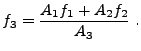
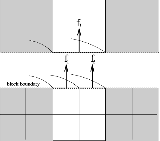
As an illustrative example of the kinds of considerations necessary in curved coordinates, Figure 8.15 shows a jump in refinement along the cylindrical `$z$' direction. When performing the flux correction step at a jump in refinement, we must take into account the area of the annulus through which each flux passes to do the proper weighting. We define the cross-sectional area through which the $z$-flux passes as

$$A = \pi (r_r^2 - r_l^2) \enskip .$$ (8.99)

The flux entering the coarse cell above the jump in refinement is corrected to agree with the fluxes leaving the fine cells that border it. This correction is weighted according to the areas

$$f_3 = \frac{A_1 f_1 + A_2 f_2}{A_3} .$$ (8.100)

Figure 8.15: Diagram showing two fine cells and a coarse cell at a jump in refinement in the cylindrical `$z$' direction. The block boundary has been cut apart here for illustrative purposes. The fluxes out of the fine blocks are shown as $f_1$ and $f_2$. These will be used to compute a more accurate flux entering the coarse flux $f_3$. The area that the flux passes through is shown as the annuli at the top of each fine cell and the annulus below the coarse cell.

For fluxes in the radial direction, the cross-sectional area is independent of the height, $z$, so the corrected flux is simply taken as the average of the flux densities in the adjacent finer cells.

8.11.4.3 Spherical geometry

One or two dimensional spherical problems can be performed by specifying  

geometry = "spherical"

in the runtime parameter file.

Cell Volume in Spherical Coordinates

1-d	$\frac{4}{3} \pi (r_r^3 - r_l^3)$
2-d	$\frac{2}{3} \pi (r_r^3 - r_l^3) (\cos(\theta_l) - \cos(\theta_r))$
3-d	$\frac{1}{3} (r_r^3 - r_l^3) (\cos(\theta_l) - \cos(\theta_r)) \Delta \phi$

If the minimum radius is chosen to be zero (xmin = 0.), the left-hand boundary type should be reflecting.

8.11.4.4 Polar geometry

Polar geometry is a 2-D subset of 3-D cylindrical configuration without the “z” coordinate. Such geometry is natural for studying objects like accretion disks. This geometry can be selected by specifying  

geometry = "polar"

in the runtime parameter file.

Cell Volume in Polar Coordinates

1-d	$\pi (r_r^2 - r_l^2)$
2-d	$\frac{1}{2} (r_r^2 - r_l^2)\Delta \phi$
3-d	$\frac{1}{2} (r_r^2 - r_l^2)\Delta \phi \Delta z$ (not supported)

As in other non-Cartesian geometries, if the minimum radius is chosen to be zero (xmin = 0.), the left-hand boundary type should be reflecting.

8.11.5 Conservative Prolongation/Restriction on Non-Cartesian Grids

When blocks are refined, we need to initialize the child data using the information in the parent cell in a manner which preserves the cell-averages in the coordinate system we are using. When a block is derefined, the parent block (which is now going to be a leaf block) needs to be filled using the data in the child blocks (which are soon to be destroyed). The first procedure is called prolongation. The latter is called restriction. Both of these procedures must respect the geometry in order to remain conservative. Prolongation and restriction are also used when filling guard cells at jumps in refinement.

8.11.5.1 Prolongation

When using a supported non-Cartesian geometry, FLASH has to use geometrically correct prolongation routines. These are located in:

• source/Grid/GridMain/paramesh/Paramesh2/monotonic (for PARAMESH 2)
• source/Grid/GridMain/paramesh/interpolation/Paramesh4/prolong (for PARAMESH 4)

These paths will be be automatically added by the setup script when the -gridinterpolation=monotonic option is in effect (which is the case by default, unless -gridinterpolation=native was specified). The “monotonic” interpolation scheme used in both cases is taking geometry into consideration and is appropriate for all supported geometries.

FLASH3 Transition: Some more specific PARAMESH 2 interpolation schemes are included in the distribution and might be useful for compatibility with FLASH2:

• source/Grid/GridMain/paramesh/Paramesh2/quadratic_cartesian (for Cartesian coordinates)
• source/Grid/GridMain/paramesh/Paramesh2/quadratic_spherical (for spherical coordinates)

Other geometry types and prolongation schemes can be added in a manner analogous to the ones implemented here.

These routines could be included by specifying the correct path in your Units file, or by using appropriate -unit= flags for setup. However, their use is not recommended.

8.11.5.2 Restriction

The default restriction routines understand the supported geometries by default. A cell-volume weighted average is used when restricting the child data up to the parent. For example, in 2-d, the restriction would look like

$$\left<f\right>_{i,j} = \frac{V_{ic,jc} \left<f\right>_{ic,jc} + V... ...left<f\right>_{ic,jc+1} + V_{ic+1,jc+1} \left<f\right>_{ic+1,jc+1}} {V_{i,j}} ,$$ (8.101)

where $V_{i,j}$ is the volume of the cell with indices, $i, j$, and the $ic, jc$ indices refer to the children.