15. Hydrodynamics Units
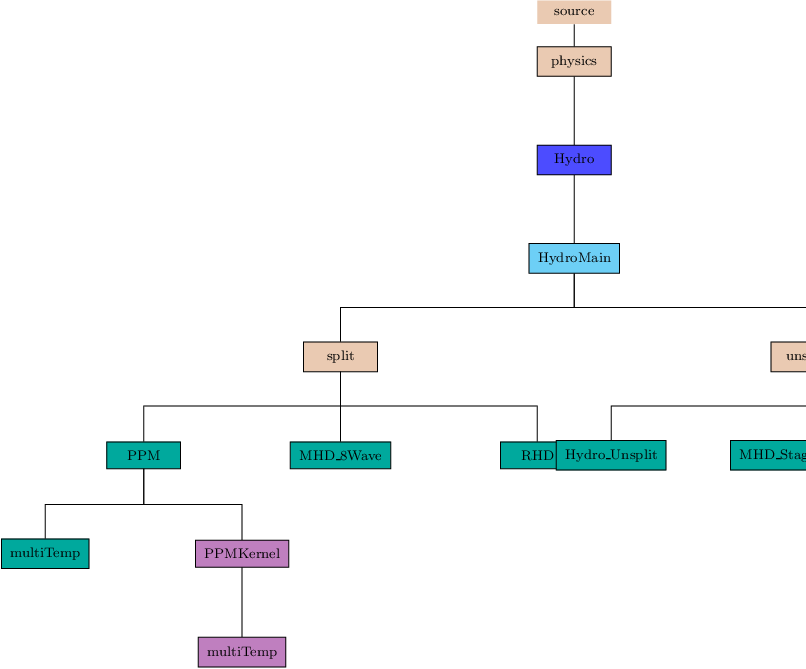
Figure 15.1:
The Hydro
unit directory tree.
|
|
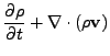
The Hydro unit solves Euler's equations for compressible gas dynamics
in one, two, or three spatial dimensions.
We first describe the basic functionality; see implementation sections
below for various extensions.
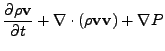
The Euler equations can be
written
in conservative form as
where  is the fluid density,
  is the fluid
velocity,
is the fluid
velocity,  is the pressure,
  is the
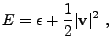
sum of the internal energy
is the
sum of the internal energy  and kinetic energy per unit mass,
 |
(15.4) |
 is the acceleration due to gravity,
and
is the acceleration due to gravity,
and  is the time coordinate.
The pressure is obtained from the energy and
density using the equation of state.
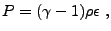
For the case of an ideal gas equation of state, the pressure is
given by
is the time coordinate.
The pressure is obtained from the energy and
density using the equation of state.
For the case of an ideal gas equation of state, the pressure is
given by
 |
(15.5) |
where  is the ratio of specific heats. More general
equations of state are discussed in Sec:Eos Gammas and Sec:Eos Helmholtz.
is the ratio of specific heats. More general
equations of state are discussed in Sec:Eos Gammas and Sec:Eos Helmholtz.
In regions where the kinetic energy greatly dominates the
total energy, computing the internal energy using
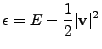 |
(15.6) |
can lead to unphysical values, primarily due to truncation error.
This results in inaccurate pressures and temperatures. To avoid this
problem, we can separately evolve the internal energy according to
![$\displaystyle \frac{\partial \rho \epsilon}{\partial t} + \nabla \cdot \left [ \left (\rho \epsilon + P \right){\bf v} \right ] - {\bf v}\cdot \nabla P = 0 .$](img659.png) |
(15.7) |
If the internal energy is a small fraction of the kinetic energy
(determined via the runtime parameter eintSwitch), then the
total energy is recomputed using the internal energy from
(15.7) and the velocities from the momentum
equation. Numerical experiments using the PPM solver included with
FLASH showed that using (15.7) when the internal
energy falls below  of the kinetic energy helps avoid the
truncation errors while not affecting the dynamics of the
simulation.
of the kinetic energy helps avoid the
truncation errors while not affecting the dynamics of the
simulation.
For reactive flows, a separate advection equation must be solved
for each chemical or nuclear species
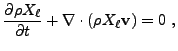 |
(15.8) |
where  is the mass fraction of the
  th species, with
the constraint that
th species, with
the constraint that
 . FLASH will enforce this
constraint if you set the runtime parameter irenorm equal to
1. Otherwise, FLASH will only restrict the abundances to fall
between smallx and 1. The quantity
. FLASH will enforce this
constraint if you set the runtime parameter irenorm equal to
1. Otherwise, FLASH will only restrict the abundances to fall
between smallx and 1. The quantity
 represents
the partial density of the th fluid. The code does not
explicitly track interfaces between the fluids, so a small amount of
numerical mixing can be expected during the course of a calculation.
represents
the partial density of the th fluid. The code does not
explicitly track interfaces between the fluids, so a small amount of
numerical mixing can be expected during the course of a calculation.
The hydro unit has a capability to advect mass scalars.
Mass scalars are field variables advected with density, similar to
species mass fractions,
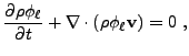 |
(15.9) |
where  is the th mass scalar.
Note that mass scalars are optional variables; to include them
specify the name of each mass scalar in a Config
file using the MASS_SCALAR keyword.
Mass scalars
are not renormalized in order to sum to
1, except when they are declared to be part of a renormalization group.
See Sec:ConfigFileSyntax
for more details.
is the th mass scalar.
Note that mass scalars are optional variables; to include them
specify the name of each mass scalar in a Config
file using the MASS_SCALAR keyword.
Mass scalars
are not renormalized in order to sum to
1, except when they are declared to be part of a renormalization group.
See Sec:ConfigFileSyntax
for more details.
Subsections
![$\displaystyle {\partial \rho E \over \partial t} +
{\bf\nabla} \cdot \left [ \left ( \rho E + P \right ) {\bf v}
\right ]$](img652.png)