Next: 8.11 Grid Geometry Up: 8. Grid Unit Previous: 8.9 GridParticles Contents Index
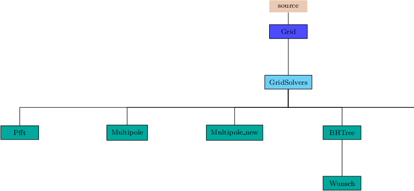
The GridSolvers unit groups together subunits that are used to solve particular types of differential equations. Currently, there are two types of solvers: a parallel Fast Fourier Transform package (Sec:GridSolversPfft) and various solvers for the Poisson equation (Sec:GridSolversPoisson).
Pfft has a layered architecture where the lower layer contains functions implementing basic tasks and primary data structures. The upper layer combines pieces from the lowest layer to interface with FLASH and create the parallel transforms. The computational part of Pfft is handled by sequential 1-dimensional FFT's, which can be from a native, vendor supplied scientific library, or from public domain packages. The current distribution of FLASH uses fftpack from NCAR for the 1-D FFTs, since that package also contains transforms that are useful with non-periodic boundary conditions.
The lowest layer has three distinct components. The first component redistributes data. It includes routines for distributed transposes for two and three dimensional data. The second component provides a uniform interface for FFT calls to hide the details of individual libraries. The third component is the data structures. There are global data structures to keep track of the type of transform, number of data dimensions, and physical and transform space information about each dimension. The dimensional information includes the start and end point of data (useful when the dimension is spread over more than one processor), the MPI communicator, the coordinates of the node in the processor grid etc. The structures also include pointers to the trigonometric tables and work space needed by the sequential FFT calls.
The upper layer of PFFT combines the lower layer routines to create end-to-end transforms in a variety of ways. The available one dimensional transforms include real-to-complex, complex-to-complex, sine and cosine transforms. They can be combined to create two or three dimensional tranforms for different configuration of the domain. The two dimensional transforms support parallelization of one dimension (or a one dimensional grid of processors). The three dimensional transforms support one or two dimensional grid of processors. All transforms must have at least one dimension within the processor at all times. The data distribution changes during the computation. However, a complete cycle of forward and inverse transform restores the data distribution.
The computation of a forward three dimensional FFT in parallel involves following steps :
The inverse transform can be computed by carrying out the steps described above in reverse order. The more commonly used domain decomposition in FFT based codes assumes a one dimensional processor grid:
During the course of a simulation, Pfft can be used in two different modes. In the first mode, every instance of Pfft use will be exactly identical to every other instance in terms of domain size and the type of transforms. In this mode, the user can set the runtime parameter pfft_setupOnce to true, which enables the FLASH initialization process to also create and initialize all the data structures of Pfft. The finalization of the Pfft subunit is also done automatically by the FLASH shutdown process in this mode. However, if a simulation needs to use Pfft in different configurations at different instances of its use, then each set of calls to Grid_pfft for computing the transforms must be preceded by a call to Grid_pfftInit and followed by a call to Grid_pfftFinalize. In addition, the runtime parameter pfft_setupOnce should be set to false. A few other helper routines are available in the subunit to allow the user to query Pfft about the dimensioning of the domain, and also to map the Mesh variables from the unk array to and from Pfft compatible (single dimensional) arrays. Pfft also provides the location of wave numbers in the parallel domain; information that users can utilize to develop their own customized PDE solvers using FFT based techniques.
The pencil grid processor topology is stored in an MPI communicator, and the communicator may contain fewer processors than are used in the simulation. This is to ensure the pencil grid points are never distributed too finely over the processors, and naturally handles the case where the user may wish to obtain a pencil grid at a very coarse level in the AMR grid. If there are more blocks than processors then we are safe to distribute the pencil grid over all processors, otherwise we must remove a number of processors. Currently, we eliminate those processors that own zero FLASH blocks at this level, as this is a simple calculation that can be computed locally.
Both mesh reconfiguration implementations generate a map describing the data movement before moving any grid data. The map is retained between calls to the Pfft routines and is only regenerated when the grid changes. This avoids repeating the same global communications, but means communication buffers are left allocated between calls to Pfft.
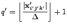
In the Collective implementation, the map coordinates are used to specify where the FLASH data is copied into a send communication buffer. Two MPI_Alltoall calls then move this data to the appropriate pencil processor at coordinates (J,K). Here, the first MPI_Alltoall moves data to processor (J,0), and the second MPI_Alltoall moves data to processor (J,K). The decision to use MPI_Alltoalls simplifies the MPI communication, but leads to very large send / receive communication buffers on each processor which consume:
Memory(bytes) = sizeof(REAL) * total grid points at solve level * 2
The PtToPt implementation consumes less memory compared to the Collective implementation, and communicates using point to point MPI messages. It is based upon using nodes in a linked list which contain metadata (a map) and a communication buffer for a single block fragment. There are two linked lists: one for the FLASH block fragments and one for Pfft block fragments. Metadata information about each FLASH block fragment is placed in separate messages and sent using MPI_Isend to the appropriate destination pencil grid processor.
Each destination pencil grid processor repeatedly invokes MPI_Iprobe using MPI_ANY_SOURCE, and creates a node in its Pfft list whenever it discovers a message. The MPI message is received into a metadata region of the freshly allocated node, and a communication buffer is also allocated according to the size specified in the metadata. The pencil processor continues probing for messages until the cumulative size of its node's communication buffers is equal to the pencil grid points it has been assigned. At this stage, grid data is communicated by traversing the Pfft list and posting MPI_Irecvs, and then traversing the FLASH list and sending block fragment using MPI_Isends. After performing MPI_Waits, the received data in the nodes of the Pfft list is copied into internal Pfft arrays.
Note, the linked list is constructed using an include file stored at flashUtilities/datastructures/linkedlist. The file is named ut_listMethods.includeF90 and is meant to be included in any Fortran90 module to create lists with nodes of a user-defined type. Please see the README file, and the unit test example at flashUtilities/datastructures/linkedlist/UnitTest.
The unit test for Pfft solver solves the following equation:
| (8.8) |
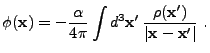
The GridSolvers subunit contains several different algorithms
for solving the general Poisson equation for a potential
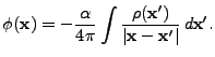
![]() given a source
given a source
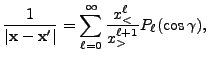
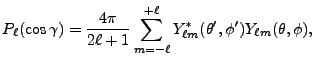
![]()
The multipole Poisson solver is appropriate for spherical or nearly-spherical
source distributions with isolated boundary conditions (Müller (1995)).
It currently works in 1D and 2D spherical, 2D axisymmetric cylindrical (![]() ), and
3D Cartesian and axisymmetric geometries. Because of the imposed symmetries,
in the 1D spherical case, only the monopole term (
), and
3D Cartesian and axisymmetric geometries. Because of the imposed symmetries,
in the 1D spherical case, only the monopole term (![]() ) makes sense,
while in the axisymmetric and 2D spherical cases, only the
) makes sense,
while in the axisymmetric and 2D spherical cases, only the ![]() moments are used (i.e., the
basis functions are Legendre polynomials).
moments are used (i.e., the
basis functions are Legendre polynomials).
The multipole algorithm consists of the following steps.
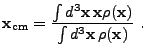
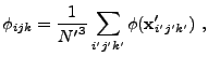
First, find the center of mass
![]()
 |
(8.10) |
| (8.13) | |||
 |
(8.14) |
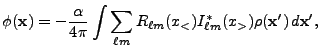
 |
 |
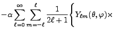
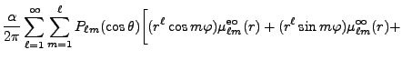
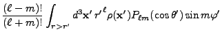
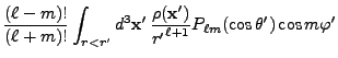
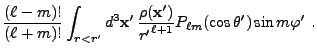
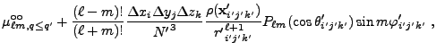
(8.16) | |
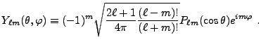
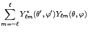
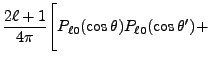
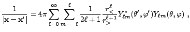
![$\displaystyle 2\sum_{m=1}^\ell {(\ell-m)!\over (\ell+m)!}
P_{\ell m}(\cos\theta)P_{\ell m}(\cos\theta')
\cos\left(m(\varphi-\varphi')\right)
\Biggr] .$](img263.png) |
In practice, the above procedure must take account of the fact that the
source and the potential are assumed to be cell-averaged
quantities discretized on a block-structured mesh with varying cell size.
Also, because of the radial dependence of the multipole moments of the
source function, these moments must be tabulated as functions of distance from
![]() , with an implied discretization. The solver allocates
storage for moment samples spaced a distance
, with an implied discretization. The solver allocates
storage for moment samples spaced a distance ![]() apart in radius
apart in radius
| (8.22) | |||
| (8.23) |
Determining the contribution of individual
cells to the tabulated moments requires some care. To reduce the error
caused by the grid geometry, in each cell ![]() an optional subgrid can be establish (see mpole_subSample)
consisting of
an optional subgrid can be establish (see mpole_subSample)
consisting of ![]() points at the locations
points at the locations
![]() , where
, where
 |
(8.24) | ||
 |
(8.25) | ||
 |
(8.26) |
 |
(8.31) |
Another way to reduce grid geometry errors when using the multipole
solver is to modify the AMR refinement criterion to refine all blocks
containing the center of mass (in addition to other criteria that may
be used, such as the second-derivative criterion supplied with PARAMESH).
This ensures that the center-of-mass point is maximally refined at all
times, further restricting the volume which contributes errors to the
moments because
![]() .
.
The default value of ![]() is 1; note that large values of this
parameter very quickly increase the amount of time required to evaluate
the multipole moments (as
is 1; note that large values of this
parameter very quickly increase the amount of time required to evaluate
the multipole moments (as ![]() ). In order to speed up the moment
summations, the sines and cosines in
((8.27))
). In order to speed up the moment
summations, the sines and cosines in
((8.27)) ![]() (8.30) are evaluated using
trigonometric recurrence relations, and the factorials are pre-computed
and stored at the beginning of the run.
(8.30) are evaluated using
trigonometric recurrence relations, and the factorials are pre-computed
and stored at the beginning of the run.
When computing the cell-averaged potential, we again employ a subgrid, but
here the subgrid points fall on cell boundaries to improve the continuity
of the result. Using ![]() subgrid points per dimension, we have
subgrid points per dimension, we have
 |
(8.32) | ||
 |
(8.33) | ||
 |
(8.34) |
 |
(8.35) |
The multipole Poisson solver is based on a multipolar expansion of the source (mass for gravity,
for example) distribution around a conveniently chosen center of expansion. The angular number
![]() entering this expansion is a measure of how detailed the description of the source
distribution will be on an angular basis. Higher
entering this expansion is a measure of how detailed the description of the source
distribution will be on an angular basis. Higher ![]() values mean higher angular resolution with
respect to the center of expansion. The multipole Poisson solver is thus appropriate for spherical
or nearly-spherical source distributions with isolated boundary conditions. For problems which
require high spatial resolution throughout the entire domain (like, for example, galaxy collision
simulations), the multipole Poisson solver is less suited, unless one is willing to go to extremely
(computationally unfeasible) high
values mean higher angular resolution with
respect to the center of expansion. The multipole Poisson solver is thus appropriate for spherical
or nearly-spherical source distributions with isolated boundary conditions. For problems which
require high spatial resolution throughout the entire domain (like, for example, galaxy collision
simulations), the multipole Poisson solver is less suited, unless one is willing to go to extremely
(computationally unfeasible) high ![]() values. For stellar evolution, however, the multipole
Poisson solver is the method of choice.
values. For stellar evolution, however, the multipole
Poisson solver is the method of choice.
The new implementation of the multipole Poisson solver is located in the directory
source/Grid/GridSolvers/Multipole_new.
The multipole Poisson solver is appropriate for spherical or nearly-spherical
source distributions with isolated boundary conditions. It currently works in
1D spherical, 2D spherical, 2D cylindrical, 3D Cartesian and 3D cylindrical. Symmetries
can be specified for the 2D spherical and 2D cylindrical cases (a horizontal symmetry plane
along the radial axis) and the 3D Cartesian case (assumed axisymmetric property).
Because of the radial symmetry in the 1D spherical case, only the monopole term
(![]() ) contributes, while for the 3D Cartesian axisymmetric, the 2D cylindrical
and 2D spherical cases only the
) contributes, while for the 3D Cartesian axisymmetric, the 2D cylindrical
and 2D spherical cases only the ![]() moments need to be used (the other
moments need to be used (the other ![]() moments effectively cancel out).
moments effectively cancel out).
The multipole algorithm consists of the following steps. First, the center of
the multipolar expansion
![]() is determined via density-squared weighted
integration over position:
is determined via density-squared weighted
integration over position:
 |
(8.36) |
 |
(8.40) | ||
 |
(8.41) |
 |
(8.44) |
| (8.45) |
We now change from complex to real formulation. We state this for the regular solid harmonic functions, the same reasoning being applied to the irregular solid harmonic functions and all their derived moments. The regular solid harmonic functions can be split into a real and imaginary part
| (8.53) | |||
| (8.54) |
| (8.55) | |||
| (8.56) |
From the above recursion relations (8.59-8.66),
the solid harmonic vector components are functions
of ![]() monomials, where
monomials, where
![]() for the
for the ![]() and (formally)
and (formally)
![]() for the
for the ![]() . For large astrophysical coordinates and large
. For large astrophysical coordinates and large ![]() values this leads
to potential computational over- and underflow. To get independent of the size of both
the coordinates and
values this leads
to potential computational over- and underflow. To get independent of the size of both
the coordinates and ![]() we introduce a damping factor
we introduce a damping factor ![]() for the coordinates
for each solid harmonic type before entering the recursions.
for the coordinates
for each solid harmonic type before entering the recursions. ![]() will be chosen such that for the
highest specified
will be chosen such that for the
highest specified ![]() we will have approximately a value close to 1 for both
solid harmonic components:
we will have approximately a value close to 1 for both
solid harmonic components:
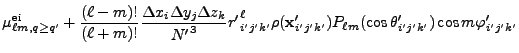
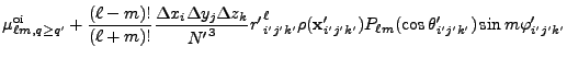
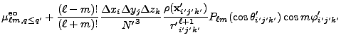
From the moment defining equations (8.48) and (8.49)
we see, that the moments are sums over subsets of cell center solid harmonic vectors multiplied
by the corresponding cell mass. From Eq.(8.57) it follows that
for highest accuracy, the moments should be calculated and stored for each possible cell face.
For high refinement levels and/or 3D simulations this would result in an unmanageable request
for computer memory. Several cell face positions have to be bundled into radial bins ![]() defined
by lower and upper radial bounds. Once a cell center solid harmonic vector pair
defined
by lower and upper radial bounds. Once a cell center solid harmonic vector pair
![]() and
and
![]() for a particular cell has been calculated, its radial bin location
for a particular cell has been calculated, its radial bin location
![]() is determined and its contribution is added to the radial bin moments
is determined and its contribution is added to the radial bin moments
![]() and
and
![]() .
The computational definition of the radial bin moments is
.
The computational definition of the radial bin moments is
How do we extract moments
![]() and
and
![]() at any particular position
at any particular position
![]() inside the domain (and, in particular, at the cell face positions
inside the domain (and, in particular, at the cell face positions ![]() ), which are
ultimately needed for the potential evaluation at that location? Assume that the location
), which are
ultimately needed for the potential evaluation at that location? Assume that the location
![]() corresponds to a particular radial bin
corresponds to a particular radial bin
![]() . Consider the
three consecutive radial bins
. Consider the
three consecutive radial bins ![]() ,
, ![]() and
and ![]() , together with their calculated moments:
, together with their calculated moments:
 |
(8.75) |
While the structure of the inner radial zone is fixed due to the underlying geometrical grid,
the size of each radial bin in the outer radial zones has to be specified by the user. There is
at the moment no automatic derivation of the optimum (accuracy vs memory cost)
bin size for the outer zones. There are two types of radial bin sizes defined for the FLASH
multipole solver: i) exponentially and/or ii) logarthmically growing:
 |
(8.80) |
| (8.81) | |||
| (8.82) |
Multithreading of the code is currently enabled in two parts: 1) during moment evaluation and 2) during potential evaluation. The threading in the moment evaluation section is achieved by running multiple threads over separate, non-conflicting radial bin sections. Moment evaluation is thus organized as a single loop over all relevant radial bins on each processor. Threading over the potential evaluation is done over blocks, as these will address different non-conflicting areas of the solution vector.
The improved multipole solver was extensively tested and several runs have been performed
using large domains (![]() ) and extremely high angular numbers up to
) and extremely high angular numbers up to ![]() for a variety
of domain geometries. Currently, the following geometries can be handled: 3D cartesian,
3D cylindrical, 2D cylindrical, 2D spherical and 1D spherical. The structure of the code is
such that addition of new geometries, should they ever be needed by some applications,
can be done rapidly.
for a variety
of domain geometries. Currently, the following geometries can be handled: 3D cartesian,
3D cylindrical, 2D cylindrical, 2D spherical and 1D spherical. The structure of the code is
such that addition of new geometries, should they ever be needed by some applications,
can be done rapidly.
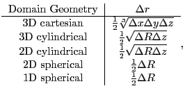
The first unit test for the multipole Poisson solver is based on the MacLaurin spheroid analytical gravitational solution given in section 35.3.4. The unit test sets up a spheroid with uniform unit density and determines both the analytical and numerical gravitational fields. The absolute relative error based on the analytical solution is formed for each cell and the maximum of all the absolute errors is compared to a predefined error tolerance value for a particular uniform refinement level. The multipole unit test runs in 2D cylindrical, 2D spherical, 3D cartesian and 3D cylindrical geometries and threaded multipole unit tests are also available.
The tree solver is based on the Barnes & Hut (1986, Nature, 324, 446) tree code for calculation of gravity forces in N-body simulations. However, it is more general and it includes some more modern features described for instance in Salmon & Warren (1994, J. Comp. Phys, 136, 155), Springel (2005, MNRAS, 364, 1105) and other works. It builds a global octal tree over the whole computational domain, communicates its part to all processors and uses it for calculations of various physical problems provided as separate units in source/physics directory. The global tree is an extension of the AMR mesh octal tree down to individual cells. The communication of the tree is implemented so that only parts of the tree that are needed for the calculation of the potential on a given processor are sent to it. The calculation of physical problems is done by walking the tree for each grid cell (hereafter point-of-calculation) and evaluating whether the tree node should be used for calculation or whether its children should be open.
The tree solver is connected to physical units by several wrapper subroutines that are called at specific places of the tree build and tree walk, and that call corresponding subroutines of physical units. In this way, physical units can include arbitrary quantity into the tree, and then, use it to calculate some other physical quantity by integrating contributions of all tree nodes during the tree walk. In this version, the only working unit implementation is physics/Gravity/GravityMain/Poisson/BHTree, which calculates the gravitational potential.
The tree solver algorithm consists of four parts. The first one, communication of block properties, is called only if the AMR grid changes. The other three, building of the tree, communication of the tree and calculation of the potential, are called in each time-step.
Communication of block properties. In recent version, each processor needs to know some basic information about all blocks in the simulation. It includes arrays: nodetype, lrefine and child. These arrays are distributed from each processor to all the other processors. They can occupy a substantial amount of memory on large number of processors (memory required for statically allocated arrays of the tree solver can be calculated by a script tree_mem_use.py).
Building the tree. The global tree is constructed from bottom and the process consists of three steps. In the first one, the so-called block-tree is constructed in each leaf block on a given processor. The block-trees are 1-dimensional dynamically allocated arrays (see Figure 8.12) and pointers to them are stored in array gr_bhTreeArray. In the second step, top nodes of block-trees (corresponding to whole blocks) are distributed to all processors and stored in array gr_bhTreeParentTree. In the last step, higher nodes of the parent tree are calculated by each processor and stored in the gr_bhTreeParentTree array. At the end, each processor holds information about the global tree down to the level of leaf blocks. During the whole process of tree building, 5 subroutines providing the interface to physical units are called: gr_bhFillBotNode, gr_bhAccBotNode, gr_bhAccNode, gr_bhNormalizeNode and gr_bhPostprocNode (see their auto-documentation and source code for details). Each of them calls a corresponding subroutine of all physical units with a name where the first two letters 'gr' are replaced with the name of the unit (e.g. Gravity_bhFillBotNode).
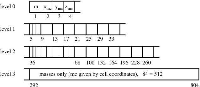 |
Communication of the tree. Most of the tree data is contained on the bottom levels in individual block-trees. In order to save memory and communication time, only parts of block-trees that are needed on a given processor are sent to it. The procedure consists of three steps. In the first one, a level down to which each block-tree has to be sent to each processor is determined. For a given block-tree, it is done by evaluating the criterion for the node acceptance (traditionally called multipole acceptance criterion, shortly MAC) for all blocks on a remote processor, searching for the maximum level down to which the evaluated node will be needed on a given remote processor. In the second step, information about the block-tree levels which are going to be communicated is sent to all processors. This information is needed for allocation of arrays in which block-trees are stored on remote processors. In the third step, the block-tree arrays are allocated, all block-trees for a given processor are packed into a single message and the messages are communicated.
The MAC is implemented in subroutine gr_bhMAC which includes only a simple geometrical MAC used also by Barnes & Hut. The node is accepted for calculation if
Tree walk. The tree is traversed from the top to the bottom, evaluating
MAC of each node and in case it is not fulfilled, continuing the tree walk with
its children. If the node's MAC is fulfilled, the node is accepted for the
calculation and subroutine gr_bhBotNodeContrib or
gr_bhNodeContrib is called, depending on whether it is a bottom-most
node (i.e. a single grid cell) or higher node, respectively. These subroutines
only call the corresponding subroutines of physical units (e.g.,
Gravity_bhNodeContrib). This is the most CPU-intensive part of
the tree solver, it usually takes more than ![]() of the total tree solver
time. It is completely parallel and it does not include any communication (apart
from sending some statistics to the main processor at the end).
of the total tree solver
time. It is completely parallel and it does not include any communication (apart
from sending some statistics to the main processor at the end).
The tree solver includes several implementations of the tree walk. The default algorithm is the Barnes-Hut like tree walk in which the whole tree is traversed from the top down to nodes fulfilling MAC for each cell separately. This algorithm is used in case the runtime parameter gr_bhUnifiedTreeWalk is true (default). If it this parameter is set to false, another algorithm is used in which instead of walking the whole tree for each cell individually, MAC is at first evaluated for whole mesh block (interacting with some node). If the node is accepted and if the node is a parent node (i.e. corresponding to whole mesh block), the node is accepted for all cells of the block and the contribution of the node is added to them. However, the node contribution is calculated separately for each cell, because the distance between the node and individual cells differs. The third tree walk algorithm is an implementation of the so called SumSquare MAC described by Salmon & Warren (1994). The tree is traversed using the priority queue, taking contribution of the most important nodes first. This algorithm provides much better error control, however, the implementation in this code version is highly experimental.
The tree solver supports isolated and periodic boundary conditions that can be set independently in each direction. In the latter case, when a node is considered for MAC evaluation and eventually calculation by calling Gravity_bhNodeContrib, periodic copies of the node are checked, and the minimum distance among the node periodic copies is taken in account. This allows for instance to calculate gravitational potential with periodic boundary conditions using the Ewald method (see description of the Gravity unit).
The unit test for the tree gravity solver calculates the gravitational potential of the Bonnor-Ebert sphere (Bonnor, W. B., 1956, MNRAS, 116, 351) and compares it to the analytical potential. The density distribution and the analytical potential are calculated by the python script bes-generator.py. The simulation setup only reads the file with radial profiles of these quantities and sets it on the grid. It also normalizes the analytical potential (adds a constant to it) so that the minimum values of the analytical and numerical potential are the same. The error of the gravitational potential calculated by the tree code is stored in the field array PERR (written into the PlotFile). The maximum absolute and relative errors are written into the log file.
This section of the User's Guide is taken from a paper by Paul Ricker, “A Direct Multigrid Poisson Solver for Oct-Tree Adaptive Meshes” (2008). Dr. Ricker wrote an original version of this multigrid algorithm for FLASH2. The Flash Center adapted it to FLASH3.
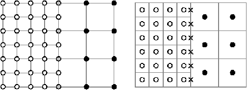
Structured adaptive mesh refinement provides some challenges for the implementation of effective, parallel multigrid methods. In the case of patch-based meshes, Huang & Greengard (2000) presents an algorithm which works by using the coarse-grid solution to impose boundary values on the fine grid. Discontinuities in the solution caused by jumps in refinement are resolved through iterative calculation of the residual and subsequent correction. While this is not a multigrid method in the standard sense, it still provides significant convergence acceleration.
The adaptation of this method to the FLASH grid structure (Ricker, 2008) requires a few modifications. The original formulation required that there be shared points between the coarse and fine patches. Contrast this with finite-volume, nested-cell, cell-averaged grids as used in FLASH(Figure 8.13). This is overcome by the exchange of guardcells from coarse to fine using monotonic interpolation (Sec:gridinterp) and external boundary extrapolation for the calculation of the residual.
|
Another difference between the method of (Ricker 2008) and Huang & Greengard is that an oct-tree undoubtedly has neighboring blocks of the same refinement, while a patch-based mesh would not. This problem is solved through uniform prolongation of boundaries from coarse-to-fine, with simple relaxation done to eliminate the slight error introduced between adjacent cells.
One final change between the two methods is that the original computes new sources at the boundary between corrections, while the propagation here is done through nested solves on various levels.
The entire algorithm requires that the PARAMESH grid be reset such that all
blocks at refinement above some level ![]() are set as temporarily nonexistent.
This is required so that guardcell filling can occur at only that level,
neglecting blocks at a higher level of refinement. This requires some global
communication by PARAMESH.
are set as temporarily nonexistent.
This is required so that guardcell filling can occur at only that level,
neglecting blocks at a higher level of refinement. This requires some global
communication by PARAMESH.
The method requires three basic operators over the solution ![]() on the grid:
taking the residual, restricting a fine-level function to coarser-level blocks,
and prolonging values from the coarse level to the faces of fine level blocks in
order to impose boundary values for the fine mesh problems.
on the grid:
taking the residual, restricting a fine-level function to coarser-level blocks,
and prolonging values from the coarse level to the faces of fine level blocks in
order to impose boundary values for the fine mesh problems.
The residual is calculated such that:
This is accomplished through the application of the finite difference laplacian,
defined on level ![]() with length-scales
with length-scales
![]() ,
,
![]() and
and
![]() .
.
| (8.85) | |||
| (8.86) |
The restriction operator
![]() for block interior zones
for block interior zones ![]() is:
is:
 |
(8.87) |
 |
(8.88) |
| (8.89) | |||
 |
|||
 |
In the case of problems with Dirichlet boundary conditions, a ![]() -dimensional
fast sine transform is used. The transform-space Green's Function for this is:
-dimensional
fast sine transform is used. The transform-space Green's Function for this is:
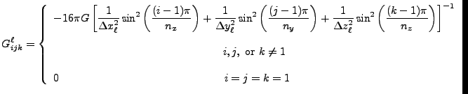
![$\displaystyle G^\ell_{ijk} = -16\pi G\left[ {1\over{\Delta x_\ell^2}}\sin^2\lef...
...) + {1\over{\Delta z_\ell^2}}\sin^2\left({k\pi\over 2n_z}\right)\right]^{-1} .$](img490.png) |
(8.90) |
However, to be able to use the block solver in a general fashion, we must be
able to impose arbitrary boundary conditions per-block. In the case of
nonhomogenous Dirichlet boundary values, boundary value elimination may be used
to generalize the solver. For instance, at the ![]() boundary:
boundary:
For periodic problems only the coarsest block must be handled differently; block adjacency for finer levels is handled naturally. The periodic solver uses a real-to-complex FFT with the Green's function:
 |
(8.92) |
This solve requires that the source be zero-averaged; otherwise the solution is non-unique. Therefore the source average is subtracted from all blocks. In order to decimate error across same-refinement-level boundaries, Gauss-Seidel relaxations to the outer two layers of zones in each block are done after applying the direct solver to all blocks on a level. With all these components outlined, the overall solve may be described by the following algorithm:
The above procedure requires storage for
![]() ,
, ![]() ,
, ![]() , and
, and ![]() on
each block, for a total storage requirement of
on
each block, for a total storage requirement of
![]() values per
block. Global communication is required in computing the tolerance-based
stopping criterion.
values per
block. Global communication is required in computing the tolerance-based
stopping criterion.
There is load imbalance in the Multigrid solver because each processor performs single block FFTs on the blocks it owns. At the coarse levels there are relatively few blocks compared to available processors which means many processors are effectively idle during the coarse level solves. The introduction of PFFT, and creation of a hybrid solver, eliminates some of the coarse level solves.
The performance characteristics of the hybrid solver are described in “Optimization of multigrid based elliptic solver for large scale simulations in the FLASH code” (2012) which is available online at http://onlinelibrary.wiley.com/doi/10.1002/cpe.2821/pdf. Performance results are obtained using the PFFT_PoissonFD unit test.
The GridSolvers subunit solves the Poisson equation ((8.9)). Two different elliptic solvers are supplied with FLASH: a multipole solver, suitable for approximately spherical source distributions, and a multigrid solver, which can be used with general source distributions. The multipole solver accepts only isolated boundary conditions, whereas the multigrid solver supports Dirichlet, given-value, Neumann, periodic, and isolated boundary conditions. Boundary conditions for the Poisson solver are specified using an argument to the Grid_solvePoisson routine which can be set from different runtime parameters depending on the physical context in which the Poisson equation is being solved. The Grid_solvePoisson routine is the primary entry point to the Poisson solver module and has the following interface
call Grid_solvePoisson (iSoln, iSrc, bcTypes(6), bcValues(2,6), poisfact) ,where iSoln and iSrc are the integer-valued indices of the solution and source (density) variables, respectively. bcTypes(6) is an integer array specifying the type of boundary conditions to employ on each of the (up to) 6 sides of the domain. Index 1 corresponds to the -x side of the domain, 2 to +x, 3 to -y, 4 to +y, 5 to -z, and 6 to +z. The following values are accepted in the array
| bcTypes | Type of boundary condition |
| 0 | Isolated boundaries |
| 1 | Periodic boundaries |
| 2 | Dirichlet boundaries |
| 3 | Neumann boundaries |
| 4 | Given-value boundaries |
When solutions found using the Poisson solvers are to be differenced (e.g., in computing the gravitational acceleration), it is strongly recommended that for AMR meshes, quadratic (or better) spatial interpolation at fine-coarse boundaries is chosen. (For PARAMESH, this is automatically the case by default, and is handled correctly for Cartesian as well as the supported curvilinear geometries. But note that the default interpolation implementation may be changed at configuration time with the '-gridinterpolation=...' setup option; and with the default implementation, the interpolation order may be lowered with the interpol_order runtime parameter.) If the order of the gridinterpolation of the mesh is not of at least the same order as the differencing scheme used in places like Gravity_accelOneRow, unphysical forces will be produced at refinement boundaries. Also, using constant or linear grid interpolation may cause the multigrid solver to fail to converge.
The poisson/multipole sub-module takes two runtime parameters,
listed in Table 8.3.
Note that storage and CPU costs scale roughly as the square of
mpole_lmax, so it is best to use this module only for nearly
spherical matter distributions.
To include the new multipole solver in a simulation, the best option
is to use the shortcut +newMpole at setup command line,
effectively replacing the following setup options :
-with-unit=Grid/GridSolvers/Multipole_new
-with-unit=physics/Gravity/GravityMain/Poisson/Multipole
-without-unit=Grid/GridSolvers/Multipole
The improved multipole solver takes several runtime parameters, whose functions are explained in detail below, together with comments about expected time and memory scaling.
| Parameter | Type | Default | Options |
| mpole_Lmax | integer | 0 | |
| mpole_2DSymmetryPlane | logical | false | true |
| mpole_3DAxisymmetry | logical | false | true |
| mpole_DumpMoments | logical | false | true |
| mpole_PrintRadialInfo | logical | false | true |
| mpole_IgnoreInnerZone | logical | false | true |
| mpole_InnerZoneSize | integer | 16 | |
| mpole_InnerZoneResolution | real | 0.1 | less than |
| mpole_MaxRadialZones | integer | 1 | |
| mpole_ZoneRadiusFraction_n | real | 1.0 | less than |
| mpole_ZoneType_n | string | ”exponential” | ”logarithmic” |
| mpole_ZoneScalar_n | real | 1.0 | |
| mpole_ZoneExponent_n | real | 1.0 | |
| real | - | any |
The tree gravity solver can be included by setup or a Config file by requesting
physics/Gravity/GravityMain/Poisson/BHTree
The current implementation works only in 3D Cartesian coordinates, and blocks have to be logically cubic (i.e., nxb=nyb=nzb). Physical dimensions of blocks can be arbitrary, however, some multipole acceptance criteria can provide inaccurate error estimates with non-cubic blocks. The computational domain can have arbitrary dimensions, and there can be more blocks with lrefine=1 (i.e., nblockx, nblocky and nblockz can have different values).
Runtime parameters gr_bhPhysMACTW and gr_bhPhysMACComm control whether MACs of physical units are used in tree walk and communication, respectively. If one of them (or both) is set .false., only purely geometric MAC is used for a corresponding part of the tree solver. It is not allowed to set gr_bhPhysMACTW = .false. and gr_bhPhysMACComm = .true..
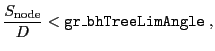
Runtime parameter gr_bhTreeLimAngle allows to set the limit opening angle for the purely geometrical MAC. Another condition controlling the acceptance of the node for the calculations is that the point-of-calculation must lie out of the box obtained by increasing the considered node by factor gr_bhTreeSafeBox.
Parameter gr_bhUseUnifiedTW controls whether the Barnes-Hut like tree
walk algorithm is used (.true.) or whether an alternative algorithm is
used which checks the MAC only once for whole block for interactions with parent
blocks (.false.; see 8.10.2.4 for more details). The latter one is ![]() faster, however, it may lead to higher errors at block boundaries, in
particular if the gravity modules calculates the potential which is
subsequently differentiated to obtain gravitational acceleration. The tree walk
algorithm base on the priority queue is used if grv_bhMAC is set to
"SumSquare".
faster, however, it may lead to higher errors at block boundaries, in
particular if the gravity modules calculates the potential which is
subsequently differentiated to obtain gravitational acceleration. The tree walk
algorithm base on the priority queue is used if grv_bhMAC is set to
"SumSquare".
| Variable | Type | Default | Description |
| gr_bhPhysMACTW | logical | .false. | whether physical MAC should be used in tree walk |
| gr_bhPhysMACComm | logical | .false. | whether physical MAC should be used in communication |
| gr_bhTreeLimAngle | real | limiting opening angle | |
| gr_bhTreeSafeBox | real | relative size of restricted volume around node where the | |
| point-of-calculation is not allowed to be located | |||
| gr_bhUseUnifiedTW | logical | .true. | whether Barnes-Hut like tree walk algorithm should be used |
| gr_bhTWMaxQueueSize | integer | .true. | maximum length of the priority queue |
The Grid/GridSolvers/Multigrid module is appropriate for general source
distributions. It solves Poisson's equation for 1, 2, and 3 dimensional
problems with Cartesian geometries. It only supports the PARAMESH
Grid with one block at the coarsest level. For any other mesh
configuration it is advisable to use the hybrid solver, which switches
to a uniform grid exact solve when the specified level of coarsening
has been achieved. In most use cases for FLASH, the multigrid solver
will be used to solve for Gravity (see: chp:Gravity). It may
be included by setup or
Config by including:
physics/Gravity/GravityMain/Poisson/Multigrid
The multigrid solver may also be included stand-alone using:
Grid/GridSolvers/Multigrid
In which case the interface is as described above. The supported boundary conditions for the module are periodic, Dirichlet, given-value, and isolated. Due to the nature of the FFT block solver, the same type of boundary condition must be used in all directions. Therefore, only the value of bcTypes(1) will be considered in the call to Grid_solvePoisson.
The multigrid solver requires the use of two internally-used grid variables: isls and icor. These are used to store the calculated residual and solved-for correction, respectively. If it is used as a Gravity solver with isolated boundary conditions, then two additional grid variables, imgm and imgp, are used to store the image mass and image potential.
| Variable | Type | Default | Description |
| mg_MaxResidualNorm | real |
|
Maximum ratio of the norm of the residual to that of the right-hand side |
| mg_maxCorrections | integer | 100 | Maximum number of iterations to take |
| mg_printNorm | real | .true. | Print the norm ratio per-iteration |
| mpole_lmax | integer | 4 | The number of multipole moments used in the isolated case |
The hybrid solver can be used in place of the Multigrid solver for problems with
./setup unitTest/PFFT_PoissonFD -auto -3d -parfile=flash_pm_3d.par -maxblocks=800 +noio


./setup unitTest/PFFT_PoissonFD -auto -3d -parfile=flash_pm_3d.par -maxblocks=800 +noio
-without-unit=Grid/GridSolvers/Multigrid/PfftTopLevelSolve
-with-unit=Grid/GridSolvers/Multigrid
It is also possible to select a different PFFT solver variant. In that case, different combinations of boundary conditions for the Poisson problem may be supported. The HomBcTrigSolver variant supports the largest set of combinations of boundary conditions. Use the PfftSolver setup variable to choose a variant. Thus, appending PfftSolver=HomBcTrigSolver to the setup chooses the HomBcTrigSolver variant. When using the hybrid solver with the PFFT variants HomBcTrigSolver or SimplePeriodicSolver, the runtime parameter gr_pfftDiffOpDiscretize should be set to 1.
The Multigrid runtime parameters given in the previous section also apply.
Grid_advanceDiffusion is the API function which solves the system of equations. This API is provided by both
the split and unsplit solvers. The unsplit solver uses HYPRE to solve the system of equations and split solver does
a direct inverse using Thomas algorithm. Note that the split solver relies heavily on PFFT infrastructure
for data exchange and a significant portion of work in split Grid_advanceDiffusion involves PFFT routines. In the
unsplit solver the data exchange is implicitly done within HYPRE and is hidden.
The steps in unsplit Grid_advanceDiffusion are as follows:
Mapping UG grid to HYPRE matrix is trivial, however mapping PARAMESH grid to a HYPRE matrix can be quite complicated. The process is simplified using the grid interfaces provided by HYPRE.
The choice of an interface is tightly coupled to the underlying grid on which the problem is being solved. We have chosen the SSTRUCT
interface as it is the most compatible with the block structured AMR mesh in FLASH4. Two terms commonly used in HYPRE terminology
are part and box. We define these terms in equivalent FLASH4 terminology. A HYPRE box object maps directly to a leaf block in FLASH4.
The block is then defined by it's extents. In FLASH4 this information can be computed easily using a combination of Grid_getBlkCornerID
and Grid_getBlkIndexLimits.All leaf blocks at a given refinement level form a HYPRE part. So number of parts in a typical
FLASH4 grid would be give by,
nparts = leaf_block(lrefine_max) - leaf_block(lrefine_min) + 1
So, if a grid is fully refined or UG, nparts = 1. However, there could still be more then one box object.
Setting up the HYPRE grid object is one of the most important step of the solution process. We use the SSTRUCT interface
provided in HYPRE to setup the grid object. Since the HYPRE Grid object is mapped directly with FLASH4 grid, whenever the
FLASH4 grid changes the HYPRE grid object needs to be updated. Consequentlywith AMR the HYPRE grid setup might happen multiple times.
Setting up a HYPRE grid object is a two step process,
Stenciled relationships typically exist between leaf blocks at same refinement level (intra part) and graph relationships exist
between leaf blocks at different refinement levels (inter part). The
fine-coarse boundary is handled in such a way that fluxes are
conserved at the interface (see Chp:diffuse for details). UG
does not require any graph relationships.
Whether a block needs a graph relationship depends on the refinement
level of it's neighbor. While this information is not directly
available in PARAMESH, it is possible to determine whether the block
neighbor is coarser or finer. Combining this information with the
constraint of at best a factor of two jump in refinement at block
boundaries, it is possible to compute the
part number of a neighbor block, which in turn determines whether we need a graph. Creating a graph involves creating a link between all the cells on
the block boundary.
Once the grid object is created, the matrix and vector objects are
built on the grid object. The diffusion solve needs uninterpolated data from
neighbor blocks even when there is a fine-coarse boundary, therefore
it cannot rely upon the guardcell fill process.
A two step process is used to handle this situation,
With the computation of Vector B (RHS), the system can be solved using HYPRE and UNK can be updated.
| Solver | Preconditioner |
| PCG | AMG, ILU(0) |
| BICGSTAB | AMG, ILU(0) |
| GMRES | AMG, ILU(0) |
| AMG | - |
| SPLIT | - |
Parallel runs: One issue that has been observed is that there is a difference in the results produced by HYPRE using one or
more processors. This would most likely be due to use of CG (krylov subspace methods), which involves an MPI_SUM over the
dot product of the residue. We have found this error to be dependent on the type of problem. One way to get across this problem is to use
direct solvers in HYPRE like SPLIT. However we have noticed that direct solvers tend to be slow. THe released code has
an option to use the SPLIT solver, but this solver has not been extensively tested and was used only for internal debugging
purposes and the usage of the HYPRE SPLIT solver in FLASH4 is purely experimental.
Customizing solvers: HYPRE exposes a lot more parameters to tweak the solvers and preconditioners mentioned above. We have only used those
which are applicable to general diffusion problems. Although in general these settings might be good enough it is by no means complete and
might not be applicable to all class of problems. Use of additional HYPRE parameters might require direct manipulation of FLASH4 code.
Symmetric Positive Definite (SPD) Matrix: PCG has been noticed to have convergence issues which might be related to (not necessarily),
The default settings use PCG as the solver with AMG as preconditioner. The following parameters
can be tweaked at run time,
| Variable | Type | Default | Description |
| gr_hyprePCType | string | "hypre_amg" | Algebraic Multigrid as Preconditioner |
| gr_hypreMaxIter | integer | 10000 | Maximum number of iterations |
| gr_hypreRelTol | real |
|
Maximum ratio of the norm of the residual to that of the initial residue |
| gr_hypreSolverType | string | "hypre_pcg" | Type of linear solver, Preconditioned Conjugate gradient |
| gr_hyprePrintSolveInfo | boolean | FALSE | enables/disables some basic solver information (for e.g number of iterations) |
| gr_hypreInfoLevel | integer | 1 | Verbosity level of solver diagnostics (refer HYPRE manual). |
| gr_hypreFloor | real |
|
Used to floor the end solution. |
| gr_hypreUseFloor | boolean | TRUE | whether to apply gr_hypreFloor to floor results from HYPRE. |
Often the systems of equations that we want to solve with HYPRE are some variation of parabolic PDES that can be expressed genericaly as
Typically these derivatives need to be discretized in the same manner independent of the system of equations with the only differences
being in the factors and transport coefficients used in the tensors ![]() ,
, ![]() ,
, ![]() ,
, ![]() ,
, ![]() &
& ![]() .
FLASH4.8 introduces a unified HYPRE solver that will construct all the necessary HYPRE objects, solve the system equations given
the tensors in Eq. 8.93, and update the Grid variables. This is supported for uniform and paramesh grids.
.
FLASH4.8 introduces a unified HYPRE solver that will construct all the necessary HYPRE objects, solve the system equations given
the tensors in Eq. 8.93, and update the Grid variables. This is supported for uniform and paramesh grids.
Previous versions of the HYPRE solvers, as described above, shared a single instance of all the HYPRE objects. The unified
solver described in this section maintains separate objects for each solver that are maintained in source/Grid/GridSolvers/HYPRE/Unified/gr_uhypreData.
New solvers are registered at setup in source/Grid/GridSolvers/HYPRE/Unified/Config. This will also generate runtime parameters
unique to each solver as described in Table 8.6 replacing gr_hypre
![]() gr_hypreSolver_.
gr_hypreSolver_.
| Parameter | Type | Default | Description |
| SolverType | STRING | "HYPRE_PCG" | Runtime parameters used with Grid/GridSolvers/HYPRE. |
| PCType | STRING | "HYPRE_AMG" | Algebraic Multigrid as Preconditioner |
| RelTol | REAL | 1.0e-8 | Maximum ratio of the norm of the residual to that of the initial residue |
| AbsTol | REAL | 0.0 | |
| SolverAutoAbsTolFact | REAL | 0.0 | |
| MinIter | INTEGER | 0 | Minimum number of iterations for HYPRE solve phase |
| MaxIter | INTEGER | 500 | Maximum number of iterations for HYPRE solve phase |
| PrintSolveInfo | BOOLEAN | FALSE | When .true. prints solve info from HYPRE |
| InfoLevel | INTEGER | 1 | level of output when using PrintSolveInfo |
| FloorType | INTEGER | 0 | |
| Floor | REAL | 1.0e-12 | Used to floor the end solution. |
| Use2Norm | BOOLEAN | FALSE | |
| CfTol | REAL | 0.0 | |
| RecomputeResidual | BOOLEAN | FALSE | |
| RecomputeResidualP | INTEGER | -1 | |
| RelChange | BOOLEAN | FALSE | |
| SlopeLimType | STRING | "HYPRESL_MC" |
Systems are solved with calls to Grid_advanceImplicit by passing an instance of parabolicProblemParms from the Grid_parabolicProblem module, whose parameters are detailed in Table 8.8. This type contains all the information about the system of equations described by Eq. 8.93. The various tensors are described by multidimensional arrays, such as FactorE whose elements will also be multiplied by a variable in unk through iFactorE, which should match the index in iFactorBMap.
| Variable | Type | Description |
| iFactorBMap | integer(ncoeffs) | Unique indices in solnvec for transport coefficients |
| iFactorA | integer(nvars) | Stores indices into solnvec for LHS term (weighting factors) |
| FactorA | real(nvars) | Constant coefficient for LHS term (weighting factor) |
| iFactorB | integer(nvars,nvars,NDIM,NDIM) | Indices in iFactorBMap for transport coefficients |
| FactorB | real(nvars,nvars,NDIM,NDIM) | Constant coefficients for transport/gradient terms |
| iFactorC | integer(nvars,nvars) | Indices in solnvec with inter variable coupling coefficients |
| FactorC | real(nvars,nvars) | Constant coefficients for coupling coefficients |
| iFactorD | integer(nvars) | Indices in solnvec to map to |
| FactorD | real(nvars) | Constant coefficient for each variable to multiply constant source |
| iFactorE | integer(nvars,nvars,NDIM) | Indices in solnvec to map to |
| FactorE | real(nvars,nvars,NDIM) | Constant coefficients for transport/gradient terms involving geometric source terms |
| iFactorF | integer(nvars,nvars,NDIM) | Indices in solnvec to map to |
| FactorF | real(nvars,nvars,NDIM) | Constant coefficients for transport/gradient terms involving geometric source terms |
| iFactorG | integer(nvars,nvars) | Indices in solnvec with inter variable coupling coefficients |
| FactorG | real(nvars,nvars) | Constant coefficients for coupling coefficients |
| iVar | integer(nvars) | Stores indices into solnvec for variables to solve |
| iFluxMap | integer(nvars) | Stores unique indices into solnvec for flux limiting variable |
| iFlux | integer(nvars) | Stores indices in iFluxMap for each variable's maximum flux |
| Flux | real(nvars) | Stores indices in iFluxMap for each variable's maximum flux |
| mode | integer(nvars) | Flux limiter mode to use for each variable |
| bcTypes | integer(NDIM,nvars,2) | Boundary condition flag |
| bcValues | real(NDIM,nvars,2) | Value or slope at boundary - when using Neumann or Dirichlet BC's |
| theta | real | Implicitness of solve |
| iSolution | integer | Handle so we can keep track of what equation we are solving. Should match a system PPDEFINE from GridSolvers/HYPRE/Unified/Config |
Eq. 8.93 is evolved with a finite-volume discretization. We integrate Eq. 8.93 over a control volume ![]() , centered
on the point
, centered
on the point
![]() , to get
, to get
where the divergence theorem has been used to turn the ![]() -factor term to be an integral over the face of our control volume and
any remaining volume integrals are approximated by the value at the center of control volume
-factor term to be an integral over the face of our control volume and
any remaining volume integrals are approximated by the value at the center of control volume
![]() . The
. The ![]() -factors
require derivatives integrated over the faces of mesh and the
-factors
require derivatives integrated over the faces of mesh and the ![]() -factors need derivatives evaluated at the cell-centers.
-factors need derivatives evaluated at the cell-centers.
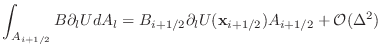
There are two classes of derivatives that could be need at a face, either derivatives normal to the face or those that are transverse to the face. In both cases finite-difference weights on a stencil of neighboring points are used, but differ in the approximation used for the surface integration. In the case of normal derivatives the stencil is constructed from cells that share the face of interest, and the derivative is evaluated at the center of the face, allowing a mid-point quadrature for the surface integral on that face.
A stencil that could approximate derivatives transverse to a cell-face would require neighboring cells that share a common edge, introducing
a new coupling between diagnoal elements, for example
![]() .
If the face-integrals are approximated with a mid-point quadrature, like in Eq. 8.97, the diagonal coupling, through the
face coefficients
.
If the face-integrals are approximated with a mid-point quadrature, like in Eq. 8.97, the diagonal coupling, through the
face coefficients
![]() &
&
![]() is no longer symmetric if the transport coefficients,
is no longer symmetric if the transport coefficients, ![]() , vary in space
, vary in space
| (8.96) |
The resulting systems of equations are numerically unstable, particularly when
![]() . In order to symmetrize
the discretization for these new edge-couplings we approximate the face-integrals with a two point trapezoid rule in the transverse direction
. In order to symmetrize
the discretization for these new edge-couplings we approximate the face-integrals with a two point trapezoid rule in the transverse direction
This way the edge-coupling is always symmetric through the edge-centered transport coefficients
![]() .
.
For both edge-centered and face-centered derivatives the Unified HYPRE solver computes stencil weights for all possible refinement configurations at fine-coarse boundaries and handles the creation of graph objects between parts.
For scalar systems of equations the finite-volume formulism in Eq. 8.94 naturally incorporates any grid geometry through the volume and area factors. However, for vector systems of equations, such as velocity with viscosity or magnetic field with resistive MHD, the discretization needs to account for geometric scale factors introduced through the vector calculus operators. The Unified HYPRE solver currently only handles "cylindrical" geometries, where it is often convenient to express the generic system of parabolic equations as
Just as before the second derivative ![]() &
& ![]() -factor terms can be integrated with the divergence theorem to be evaluated
on the cell-faces, but the volume
-factor terms can be integrated with the divergence theorem to be evaluated
on the cell-faces, but the volume ![]() &
& ![]() -factor terms will include a
-factor terms will include a
![]() geometric term.
geometric term.
![$\displaystyle \left[ r^\ell \int_{r<r'} d^3{\bf x}' {\rho({\bf x}')
Y_{\ell m}^...
...x}' \rho({\bf x}')
Y_{\ell m}^*(\theta',\varphi') {r'}^\ell \right]\Biggr\} .$](img259.png)
![$\displaystyle -{\alpha\over 4\pi}
\sum_{\ell=0}^\infty P_{\ell 0}(\cos\theta)\l...
...u^{\rm eo}_{\ell 0}(r) +
{1\over r^{\ell+1}} \mu^{\rm ei}_{\ell 0}(r) \right] -$](img264.png)
![$\displaystyle \qquad\qquad\qquad\qquad\qquad
{\cos m\varphi\over r^{\ell+1}} \m...
...ell m}(r) +
{\sin m\varphi\over r^{\ell+1}} \mu^{\rm oi}_{\ell m}(r) \biggr] .$](img266.png)

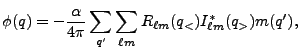
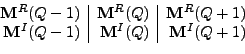
![$\displaystyle \phi({\bf x}_F) = -{\alpha\over 4\pi} \sum_{q'} \sum_{\ell m}R_{\ell m}([q',x_F]_<)I_{\ell m}^*([q',x_F]_>)m(q'),$](img348.png)
![$\displaystyle \phi({\bf x}_F) = -{\alpha\over 4\pi}\left\{ \sum_{q'\leq x_F} \s...
...} \sum_{\ell m}R_{\ell m}({\bf x}_F)\left[I_{\ell m}^*(q')m(q')\right]\right\},$](img353.png)
![$\displaystyle \phi({\bf x}_F) = -{\alpha\over 4\pi}\left[ \sum_{\ell m}M^R_{\el...
...\bf x}_F) + \sum_{\ell m}M^{I*}_{\ell m}({\bf x}_F)R_{\ell m}({\bf x}_F)\right]$](img358.png)
![$\displaystyle \phi({\bf x}_F) = -{\alpha\over 4\pi}\left\{ \left[\begin{array}{...
...ay}{l} {\bf R}^c({\bf x}_F) {\bf R}^s({\bf x}_F) \end{array}\right]\right\},$](img370.png)
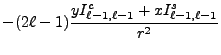
![$\displaystyle {(2\ell - 1)zI_{\ell-1,m}^{c/s}-\left[(\ell-1)^2-m^2\right]
I_{\ell-2,m}^{c/s}\over r^2},\;\;\;0\leq m <\ell$](img388.png)
![$\displaystyle {1\over r}{L\over e}\sqrt[2L]{2\pi L}$](img420.png)
![$\displaystyle {1\over r}{L\over e}\sqrt[2L+2]{{2\pi e^2\over L}},$](img422.png)

![$\displaystyle V_\alpha A_i \left . \frac{\partial U_i}{\partial t} \right \vert...
...a D_i + \left [ V_\alpha F_{ijk} \partial_k U^*_j \right ]_{\mathbf{x}_\alpha},$](img548.png)