Next: 35.4 Particles Test Problems Up: 35. The Supplied Test Previous: 35.2 Magnetohydrodynamics Test Problems Contents Index
The Jeans problem allows one to examine the behavior of sinusoidal,
adiabatic
density perturbations in both the pressure-dominated and gravity-dominated
limits. This problem uses periodic boundary conditions.
The equation of state is that of a perfect gas.
The initial conditions at ![]() are
are
 |
(35.31) |
 |
(35.32) |
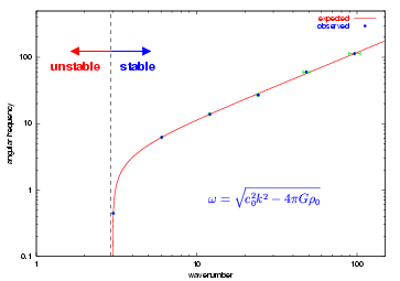
We checked the dispersion relation (35.33) for stable perturbations with
![]() by fixing
by fixing
![]() and
and ![]() and performing several runs with different
and performing several runs with different ![]() .
We followed each case for roughly five oscillation periods using a
uniform grid in the box
.
We followed each case for roughly five oscillation periods using a
uniform grid in the box ![]() . We used
. We used
![]() g cm
g cm![]() and
and
![]() dyn cm
dyn cm![]() ,
yielding
,
yielding
![]() cm
cm![]() . The perturbation amplitude
. The perturbation amplitude
![]() was fixed at
was fixed at ![]() . The box size
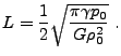
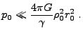
. The box size ![]() is chosen so that
is chosen so that
![]() is smaller than the smallest nonzero wavenumber that can be
resolved on the grid
is smaller than the smallest nonzero wavenumber that can be
resolved on the grid
 |
(35.34) |
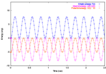
The resulting kinetic, thermal, and potential energies as functions
of time for one choice of ![]() are shown in Figure 35.58 together with the analytic solution, which is given in two
dimensions by
are shown in Figure 35.58 together with the analytic solution, which is given in two
dimensions by
|
|
| Variable | Type | Default | Description | ||||
| rho0 | real |
|
Initial unperturbed density ( |
||||
| p0 | real |
|
Initial unperturbed pressure ( |
||||
| amplitude | real | 0.001 | Perturbation amplitude ( |
||||
| lambdax | real | 0.572055 | Perturbation wavelength in |
||||
| lambday | real |
|
Perturbation wavelength in |
||||
| lambdaz | real |
|
Perturbation wavelength in |
||||
| delta_ref | real | 0.01 | Refine a block if the maximum density
contrast relative to
|
||||
| delta_deref | real | -0.01 | Derefine a block if the maximum density
contrast relative to
|
||||
| reference_density | real |
|
Reference density for grid refinement
(
|
The additional runtime parameters supplied with the Jeans problem are listed in Table 35.10. This problem is configured to use the perfect-gas equation of state (gamma) with gamma set to 1.67 and is run in a two-dimensional unit box. The refinement marking routine (Grid_markRefineDerefine.F90) supplied with this problem refines blocks whose mean density exceeds a given threshold. Since the problem is not spherically symmetric, the multigrid Poisson solver should be used.
The homologous dust collapse problem DustCollapse is used to test the ability of the code to solve self-gravitating problems in which the flow geometry is spherical and gas pressure is negligible. The problem was first described by Colgate and White (1966) and has been used by Mönchmeyer and Müller (1989) to test hydrodynamical schemes in curvilinear coordinates. We solve this problem using a 3D Cartesian grid.
The initial conditions consist of a uniform sphere of radius ![]() and
density
and
density ![]() at rest. The pressure
at rest. The pressure ![]() is taken to be constant and
very small
is taken to be constant and
very small
 |
(35.36) |
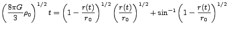
The collapse of the dust sphere is self-similar; the cloud should remain
spherical with uniform density as it collapses. The radius of the cloud,
![]() , should satisfy
, should satisfy
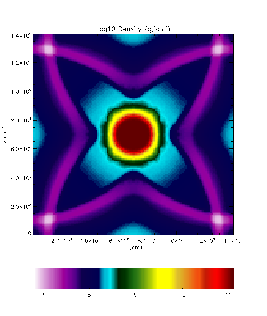
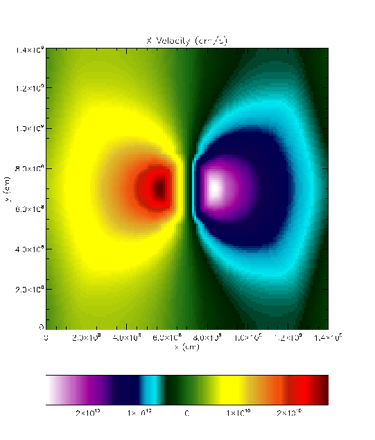
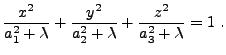
Results of a DustCollapse run using FLASH 3.0 appear in
Figure 35.60, which shows plots of density and the X
component of velocity in menacing color scheme. The values are plotted
at the end of the run from an X-Y plane in the center of the physical
domain; density is in logarithmic scale. This run used a resolution of
![]() , and the results were compared against a similar run using
FLASH 2.5. We have also included figures from an earlier higher
resolution run using FLASH2 which used
, and the results were compared against a similar run using
FLASH 2.5. We have also included figures from an earlier higher
resolution run using FLASH2 which used ![]() top-level blocks and
seven levels of refinement, for an effective resolution of
top-level blocks and
seven levels of refinement, for an effective resolution of ![]() .
In both the runs, the multipole Poisson solver was used with a maximum
multipole moment
.
In both the runs, the multipole Poisson solver was used with a maximum
multipole moment ![]() . The initial conditions used
. The initial conditions used
![]() g cm
g cm![]() and
and
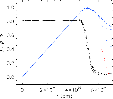
![]() cm. In Figure 35.61a, the density, pressure, and velocity are scaled by
cm. In Figure 35.61a, the density, pressure, and velocity are scaled by
![]() g cm
g cm![]() ,
,
![]() dyn cm
dyn cm![]() , and
, and
![]() cm s
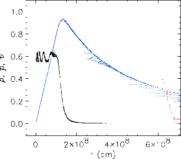
cm s![]() , respectively. In Figure 35.61b they are scaled by
, respectively. In Figure 35.61b they are scaled by
![]() g cm
g cm![]() ,
,
![]() dyn cm
dyn cm![]() , and
, and
![]() cm s
cm s![]() . Note that within the cloud, the
profiles are very isotropic, as indicated by the small dispersion in
each profile. Significant anisotropy is only present for low-density
material flowing in through the Cartesian boundaries. In particular,
it is encouraging that the velocity field remains isotropic all the
way into the center of the grid; this shows the usefulness of
refining spherically symmetric problems near
. Note that within the cloud, the
profiles are very isotropic, as indicated by the small dispersion in
each profile. Significant anisotropy is only present for low-density
material flowing in through the Cartesian boundaries. In particular,
it is encouraging that the velocity field remains isotropic all the
way into the center of the grid; this shows the usefulness of
refining spherically symmetric problems near ![]() . However, as
material flows inward past refinement boundaries, small ripples
develop in the density profile due to interpolation errors. These
remain spherically symmetric but increase in amplitude as they are
compressed. Nevertheless, they are still only a few percent in
relative magnitude by the second frame. The other numerical effect
of note is a slight spreading at the edge of the cloud. This does
not appear to worsen significantly with time. If one takes the
radius at which the density drops to one-half its central value as
the radius of the cloud, then the observed collapse factor agrees
with our expectation from (35.37). Overall our
results, including the numerical effects, agree well with those of
Mönchmeyer and Müller (1989).
. However, as
material flows inward past refinement boundaries, small ripples
develop in the density profile due to interpolation errors. These
remain spherically symmetric but increase in amplitude as they are
compressed. Nevertheless, they are still only a few percent in
relative magnitude by the second frame. The other numerical effect
of note is a slight spreading at the edge of the cloud. This does
not appear to worsen significantly with time. If one takes the
radius at which the density drops to one-half its central value as
the radius of the cloud, then the observed collapse factor agrees
with our expectation from (35.37). Overall our
results, including the numerical effects, agree well with those of
Mönchmeyer and Müller (1989).
This problem is configured to use the perfect-gas equation of state (gamma) with gamma set to 1.67 and is run in a three-dimensional box. The problem uses the specialized refinement marking routine supplied under the Grid interface of Grid_markRefineSpecialized which refines blocks containing the center of the cloud.
|
[]  []
[] 
|
|
[]  []
[] 
|
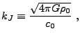
The PoisTest problem tests the convergence properties of the multigrid Poisson solver on a multidimensional, highly (locally) refined grid. This problem is described by Huang and Greengard (2000). The source function consists of a sum of thirteen two-dimensional Gaussians
![$\displaystyle \rho(x,y) = \sum_{i=1}^{13} e^{-\sigma_i[(x-x_i)^2+(y-y_i)^2]} ,$](img3899.png) |
(35.38) |
|
| 1 | 2 | 3 | 4 | 5 | 6 | 7 | |
| 0 | -1 | -1 | 0.28125 | 0.5 | 0.3046875 | 0.3046875 | |
| 0 | 0.09375 | 1 | 0.53125 | 0.53125 | 0.1875 | 0.125 | |
| 0.01 | 4000 | 20000 | 80000 | 16 | 360000 | 400000 | |
| 8 | 9 | 10 | 11 | 12 | 13 | ||
| 0.375 | 0.5625 | -0.5 | -0.125 | 0.296875 | 0.5234375 | ||
| 0.15625 | -0.125 | -0.703125 | -0.703125 | -0.609375 | -0.78125 | ||
| 2000 | 18200 | 128 | 49000 | 37000 | 18900 |
The PoisTest problem uses one additional runtime parameters sim_smlRho, the smallest allowed value of density. Runtime parameters from the Multigrid unit (both Gravity and GridSolvers) are relevant; see Sec:GridSolversMultigrid.
As a test case, an oblate (
![]() ) Maclaurin spheroid, of a constant density
) Maclaurin spheroid, of a constant density ![]() in the interior, and
in the interior, and
![]() outside (in FLASH4
smlrho is used).
The spheroid is motionless and in hydrostatic equilibrium.
The gravitational potential of such object is analytically
calculable, and is:
outside (in FLASH4
smlrho is used).
The spheroid is motionless and in hydrostatic equilibrium.
The gravitational potential of such object is analytically
calculable, and is:
| (35.39) |
 |
(35.40) | ||
 |
(35.41) |
 |
(35.42) |
![$\displaystyle \phi({\bf x}) = \frac{2a_3}{e^2} \pi G \rho \left[a_1 e \tan^{-1}...
...( \tan^{-1}h - \frac{h}{1+h^2} \right) + 2z^2 (h-\tan^{-1}h) \right) \right] ,$](img3912.png) |
(35.43) |
| (35.44) |
 |
(35.45) |
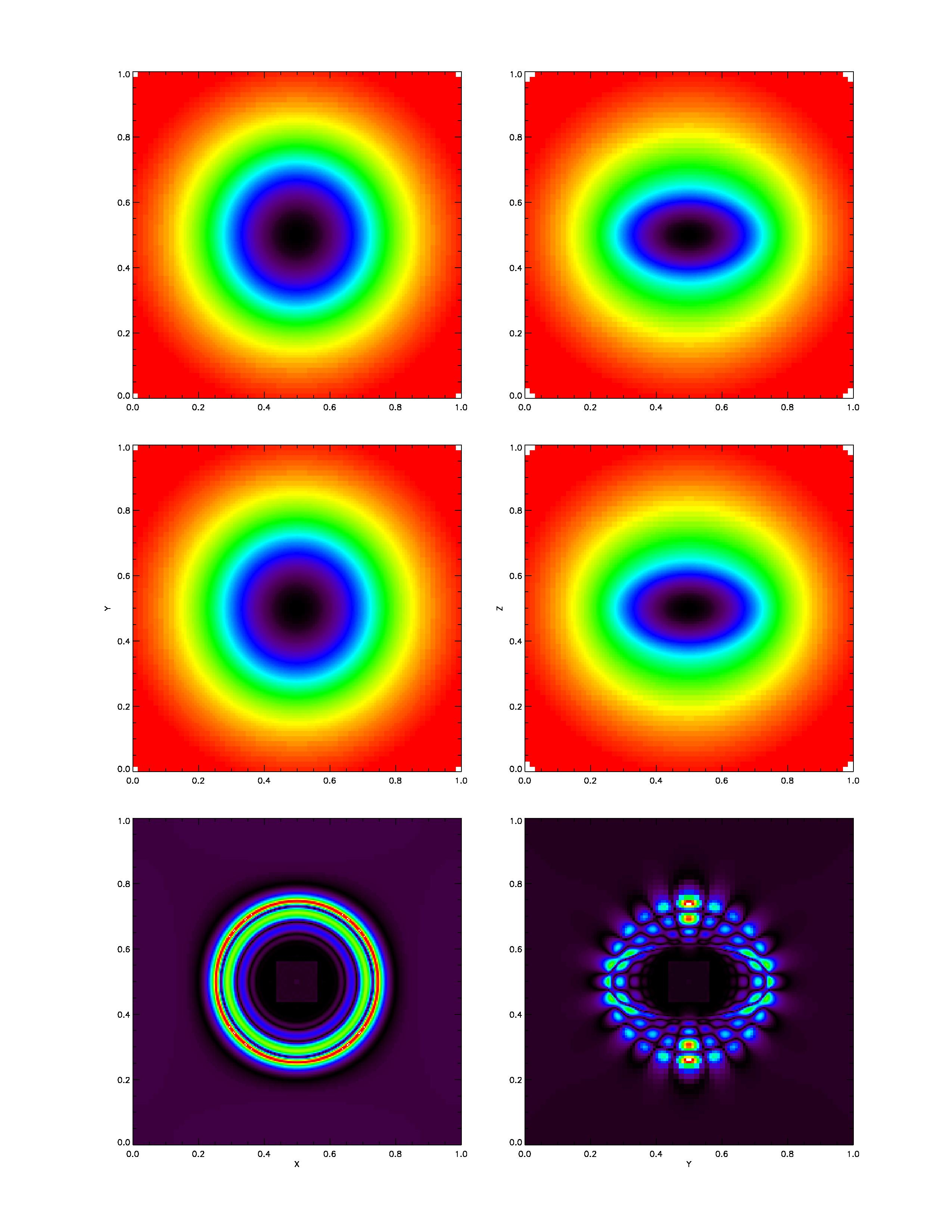
This test is also useful because the spheroid has spherical symmetry in the X-Y plane,
but also lack of such symmetry in X-Z and Y-Z planes.
The density distribution of the spheroid is shown in Figure 35.3.4.
Spherical symmetry is simple to reproduce with a solution using multipole expansion.
However, the non-symmetric solution requires
an infinite number of multipole moments, while the code
calculates solution up to a certain ![]() , specified by the user
as runtime parameter mpole_lmax. The error is thus expected to be dominated
by the first non-zero term in the remainder of expansion. Also, the solution for any point inside
the spheroid is the sum of monopole and dipole moments.
, specified by the user
as runtime parameter mpole_lmax. The error is thus expected to be dominated
by the first non-zero term in the remainder of expansion. Also, the solution for any point inside
the spheroid is the sum of monopole and dipole moments.
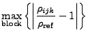
|
The simulation is calculated on a MacLaurin spheroid with eccentricity ![]() ; several other values for eccentricity were tried with results qualitatively the same.
All tests used 3D Cartesian coordinates.
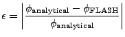
The gravitational potential is calculated on an adaptive mesh, and the relative error is investigated:
; several other values for eccentricity were tried with results qualitatively the same.
All tests used 3D Cartesian coordinates.
The gravitational potential is calculated on an adaptive mesh, and the relative error is investigated:
|
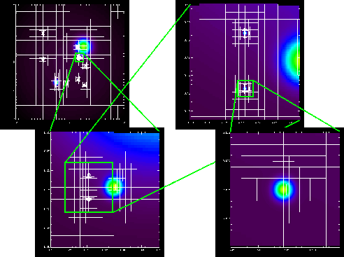
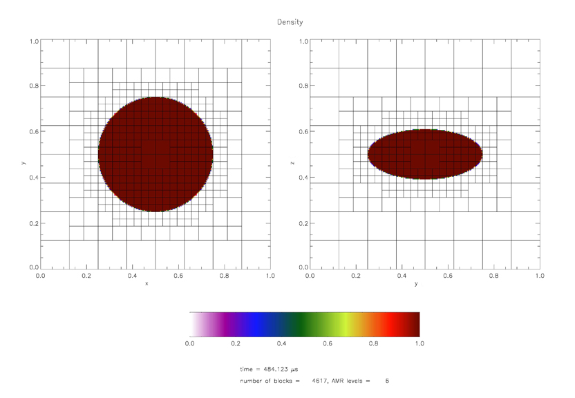
As expected, increasing spatial resolution improves the solution quality, but here we focus on
how the solution depends on the choice of ![]() , the cutoff
, the cutoff
![]() in (8.15). In Figure 35.64-35.64
the gravitational potential for the Maclaurin
spheroid, the FLASH4 solution, and relative errors for several
in (8.15). In Figure 35.64-35.64
the gravitational potential for the Maclaurin
spheroid, the FLASH4 solution, and relative errors for several ![]() 's are shown.
A similar figure produced for
's are shown.
A similar figure produced for ![]() shows no difference from Figure 35.64,
indicating that the last dipole term in the multipole expansion does not contribute to the accuracy
of the solution but does increase computational cost.
Because gravity sources are all of the same sign, and the symmetry of the
problem, all odd-
shows no difference from Figure 35.64,
indicating that the last dipole term in the multipole expansion does not contribute to the accuracy
of the solution but does increase computational cost.
Because gravity sources are all of the same sign, and the symmetry of the
problem, all odd-![]() moments are zero: reasonable, physically motivated values for
setting mpole_lmax should be an even number.
moments are zero: reasonable, physically motivated values for
setting mpole_lmax should be an even number.
In the X-Y plane, where the solution is radially symmetric, the first monopole term is enough to qualitatively capture the correct
potential. As expected, the error is the biggest on the spheroid boundary,
and decreases both outwards and inwards. Increasing the maximum included moment reduces errors.
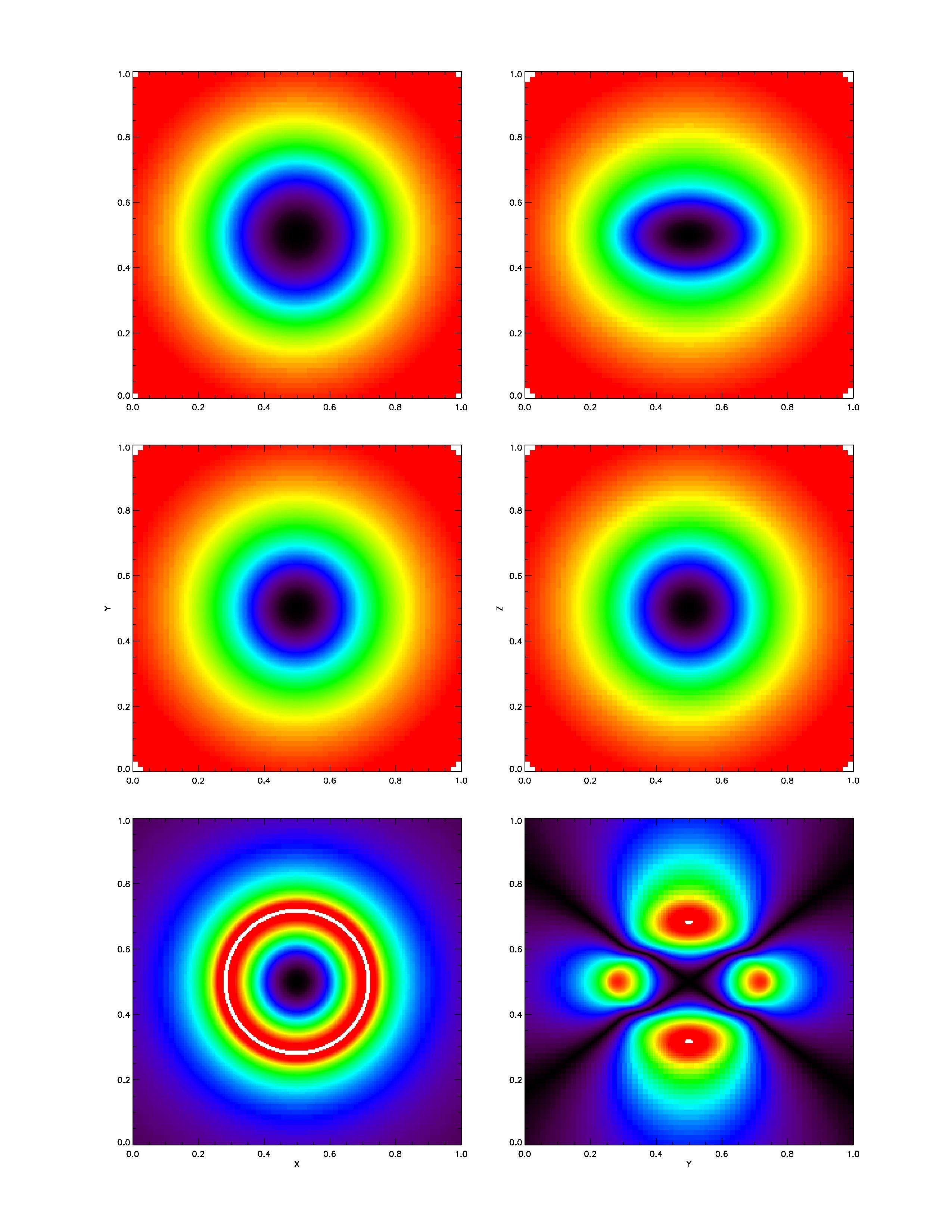
However, in other non-symmetric planes,
truncating the potential to certain ![]() leads to an error whose leading term will be
the spherical harmonic of order
leads to an error whose leading term will be
the spherical harmonic of order ![]() , as can be nicely seen in the lower right sections of
Figure 35.64 - 35.66.
Increasing
, as can be nicely seen in the lower right sections of
Figure 35.64 - 35.66.
Increasing ![]() reduces the error, but also increases the required time for computation.
This computational increase is not
linear because of the double sum in (8.17).
Luckily, convergence is rather fast, and already
for
reduces the error, but also increases the required time for computation.
This computational increase is not
linear because of the double sum in (8.17).
Luckily, convergence is rather fast, and already
for
![]() , there are only few zones with relative error bigger than 1%, while for the most of the computational domain the error is several orders of magnitude less.
, there are only few zones with relative error bigger than 1%, while for the most of the computational domain the error is several orders of magnitude less.
|
|
|
![$\displaystyle {\rho_0\delta^2\vert\omega\vert^2L^2\over 8k^2}\left[1-{\rm cos}(2\omega t)
\right]$](img3872.png)
![$\displaystyle -{\pi G\rho_0^2\delta^2L^2\over 2k^2}\left[1+{\rm cos}(2\omega t)
\right] .$](img3876.png)