Next: 35.3 Gravity Test Problems Up: 35. The Supplied Test Previous: 35.1 Hydrodynamics Test Problems Contents Index
The Brio-Wu MHD shock tube problem (Brio and Wu, 1988),
magnetoHD/BrioWu, is a
coplanar magnetohydrodynamic counterpart of the hydrodynamic Sod
problem (Sec:SimulationSod). The initial left
and right states are given by ![]() ,
, ![]() ,
, ![]() ,
,
![]() ; and
; and
![]() ,
, ![]() ,
, ![]() ,
,
![]() . In addition,
. In addition, ![]() and
and ![]() . This is a good
problem to test wave properties of a particular MHD solver, because
it involves two fast rarefaction waves, a slow compound wave, a
contact discontinuity and a slow shock wave.
. This is a good
problem to test wave properties of a particular MHD solver, because
it involves two fast rarefaction waves, a slow compound wave, a
contact discontinuity and a slow shock wave.
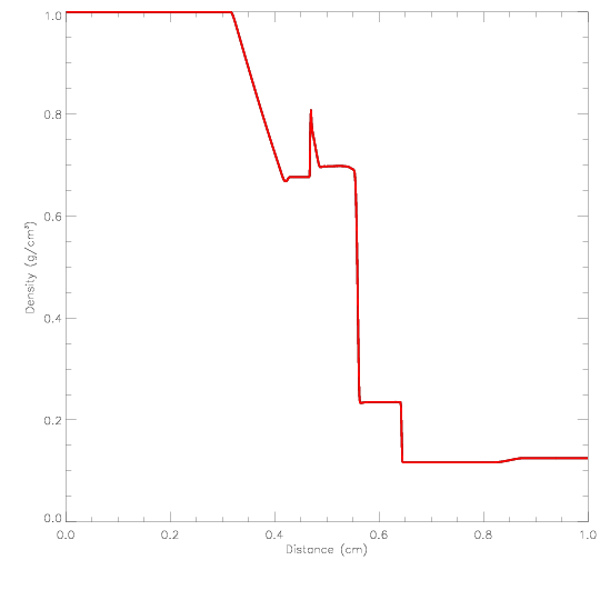
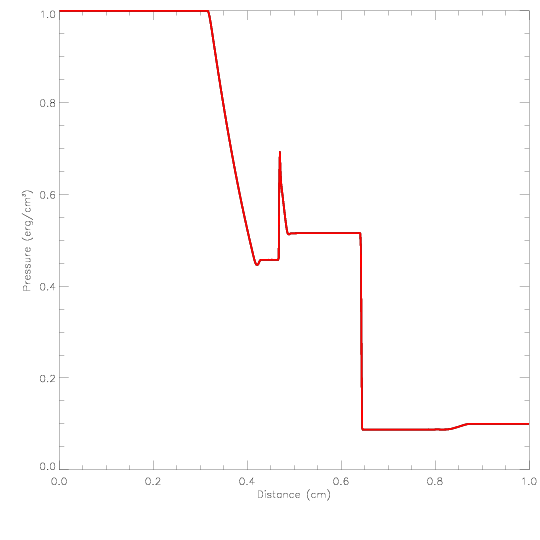
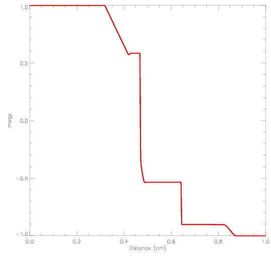
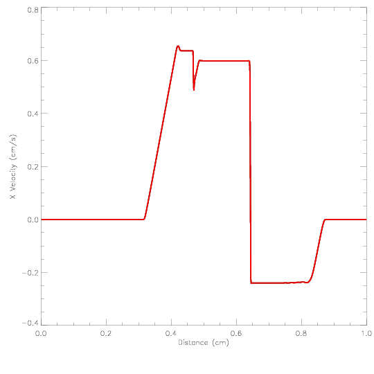
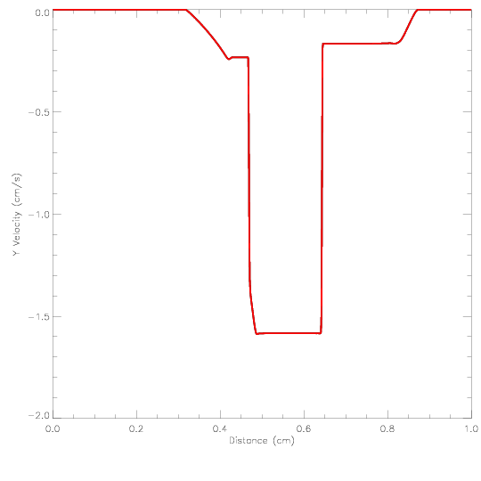
The conventional 800 point solution to this problem computed with
FLASH is presented in Figure 35.35,
Figure 35.36, Figure 35.37,
Figure 35.38, and Figure 35.39 . The figures show the
distribution of density, normal and tangential velocity components,
tangential magnetic field component and pressure at ![]() (in
non-dimensional units). As can be seen, the code accurately and
sharply resolves all waves present in the solution. There is a small
undershoot in the solution at
(in
non-dimensional units). As can be seen, the code accurately and
sharply resolves all waves present in the solution. There is a small
undershoot in the solution at
![]() , which results from a
discontinuity-enhancing monotonized centered gradient limiting
function (LeVeque 1997). This undershoot can be easily removed if a
less aggressive limiter, e.g. a minmod or a van Leer limiter,
is used instead. This, however, will degrade the sharp resolution of
other discontinuities.
, which results from a
discontinuity-enhancing monotonized centered gradient limiting
function (LeVeque 1997). This undershoot can be easily removed if a
less aggressive limiter, e.g. a minmod or a van Leer limiter,
is used instead. This, however, will degrade the sharp resolution of
other discontinuities.
The directionally splitting 8Wave MHD solver
with a second-order MUSCL-Hancock scheme (setup with +8wave) was used
for the results shown in this simulation.
The StaggeredMesh MHD solver (setup with +usm) can also be used
for this Brio-Wu problem in one- and two-dimensions.
However, in the latter case, the StaggeredMesh
solver only supports non-rotated setups for which
a shock normal is parallel to the ![]() -axis that
initially intersects that axis
at
-axis that
initially intersects that axis
at ![]() (halfway across a box with unit dimensions).
This limitation occurs in the StaggeredMesh
scheme because the currently released version of
the FLASH code does not truly support physically
correct boundary conditions for this rotated shock
geometry.
(halfway across a box with unit dimensions).
This limitation occurs in the StaggeredMesh
scheme because the currently released version of
the FLASH code does not truly support physically
correct boundary conditions for this rotated shock
geometry.
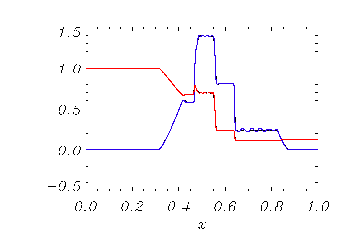
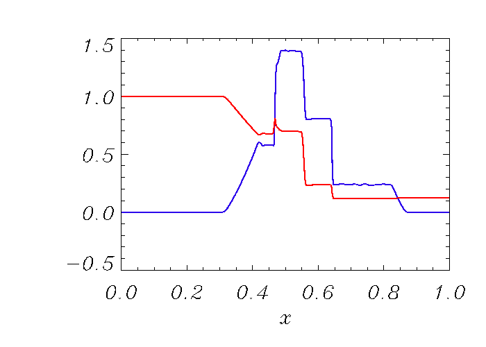
Figure 35.40 clearly demonstrates that the
conventional PPM reconstruction method fails to preserve
monotonicities, shedding oscillations especially in the plateau
near strong discontinuities such as the contact and right
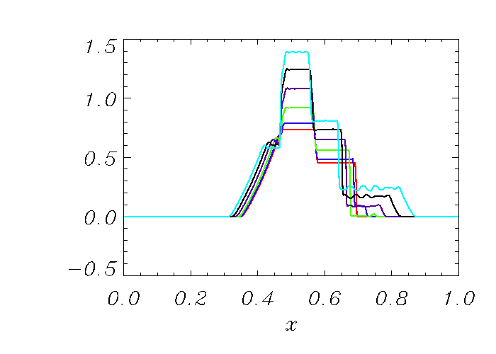
going slow MHD shock. In Fig. 35.41, Mach
numbers are plotted with varying strengths of the transverse field
![]() . The oscillations increase with an increase of
. The oscillations increase with an increase of ![]() ;
the reason being that stronger
;
the reason being that stronger ![]() introduces more transverse effect
that resists shock propagation in the
introduces more transverse effect
that resists shock propagation in the ![]() direction causing the
shock to move slowly. This effect is clearly seen in the locations of
the shock fronts (right going slow MHD shocks in this case), which
remain closer to the initial location
direction causing the
shock to move slowly. This effect is clearly seen in the locations of
the shock fronts (right going slow MHD shocks in this case), which
remain closer to the initial location ![]() when
when ![]() is
stronger.
is
stronger.
|
|
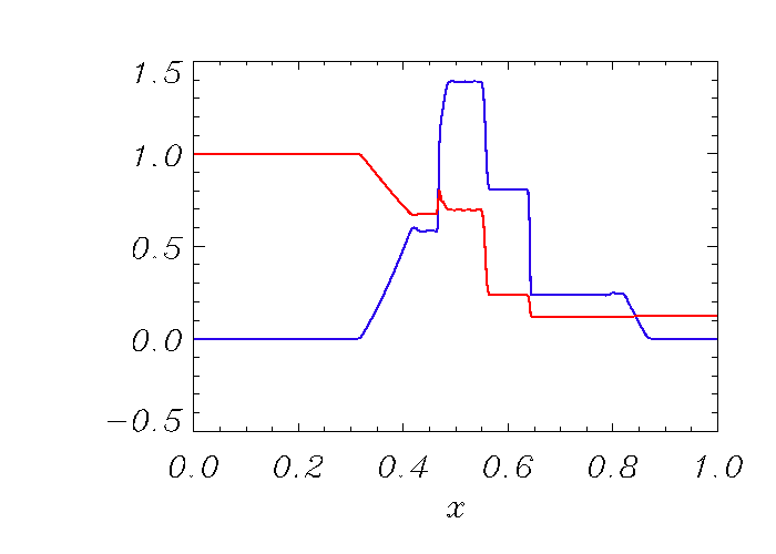
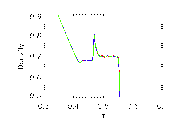
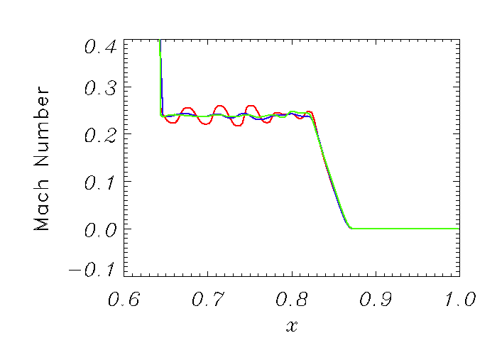
Results from using the upwind biased slope limiter for PPM are illustrated in Figures 35.42 - 35.45 . The oscillation shedding found in the conventional PPM (e.g., Fig. 35.40) are significantly reduced in both density, and Mach number profiles. The overall qualitative solution behavior of using the upwind PPM approach, shown in Fig. 35.42, is very much similar to those from the 5th order WENO method as illustrated in Fig. 35.43. As shown in the closeup views in Fig. 35.44 and 35.45, the solutions with the upwind PPM slope limiter (blue curves) outperforms the conventional PPM method (red curves), and compares well with the WENO scheme (green curves). In fact, the upwind approach shows the most flat density plateau of all methods. Note that the SMS issue can be observed regardless of the choice of Riemann solvers and the dissipation mechanism in PPM (e.g., even with flattening on). 400 grid points were used.
|
|
|
|
The Orszag-Tang MHD vortex problem (Orszag and Tang, 1979),
magnetoHD/OrszagTang, is a simple
two-dimensional problem that has become a classic test for MHD codes.
In this problem a simple, non-random initial condition is imposed at
time ![]()
| (35.17) |
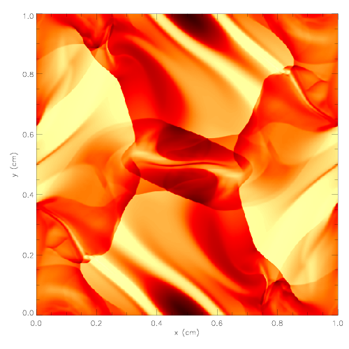
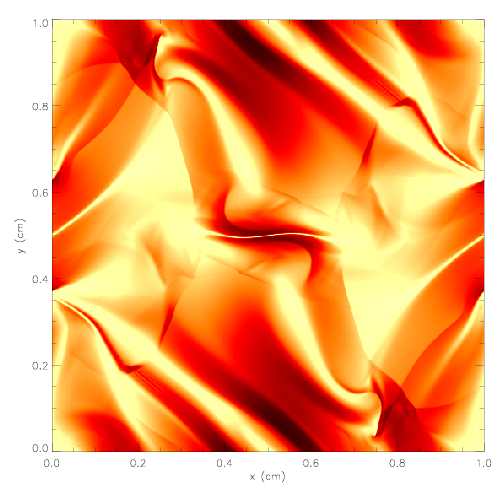
As the evolution time increases, the vortex flow pattern becomes
increasingly complicated due to the nonlinear interactions of waves.
A highly resolved simulation of this problem should produce
two-dimensional MHD turbulence. Figure 35.46 and
Figure 35.47 shows density and magnetic field
contours at ![]() . As one can observe, the flow pattern at this
time is already quite complicated. A number of strong waves have
formed and passed through each other, creating turbulent flow
features at all spatial scales.
. As one can observe, the flow pattern at this
time is already quite complicated. A number of strong waves have
formed and passed through each other, creating turbulent flow
features at all spatial scales.
The results were obtained using the directionally splitting 8Wave MHD solver for this Orszag-Tang problem.
The 3D version are also shown in the below solved using the unsplit staggered mesh MHD solver.
|
[a] 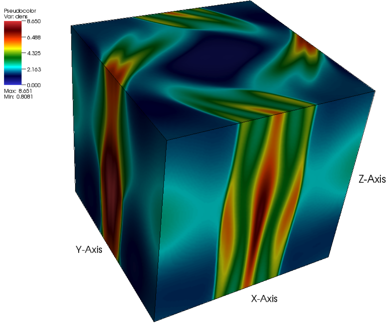 [b]
[b] 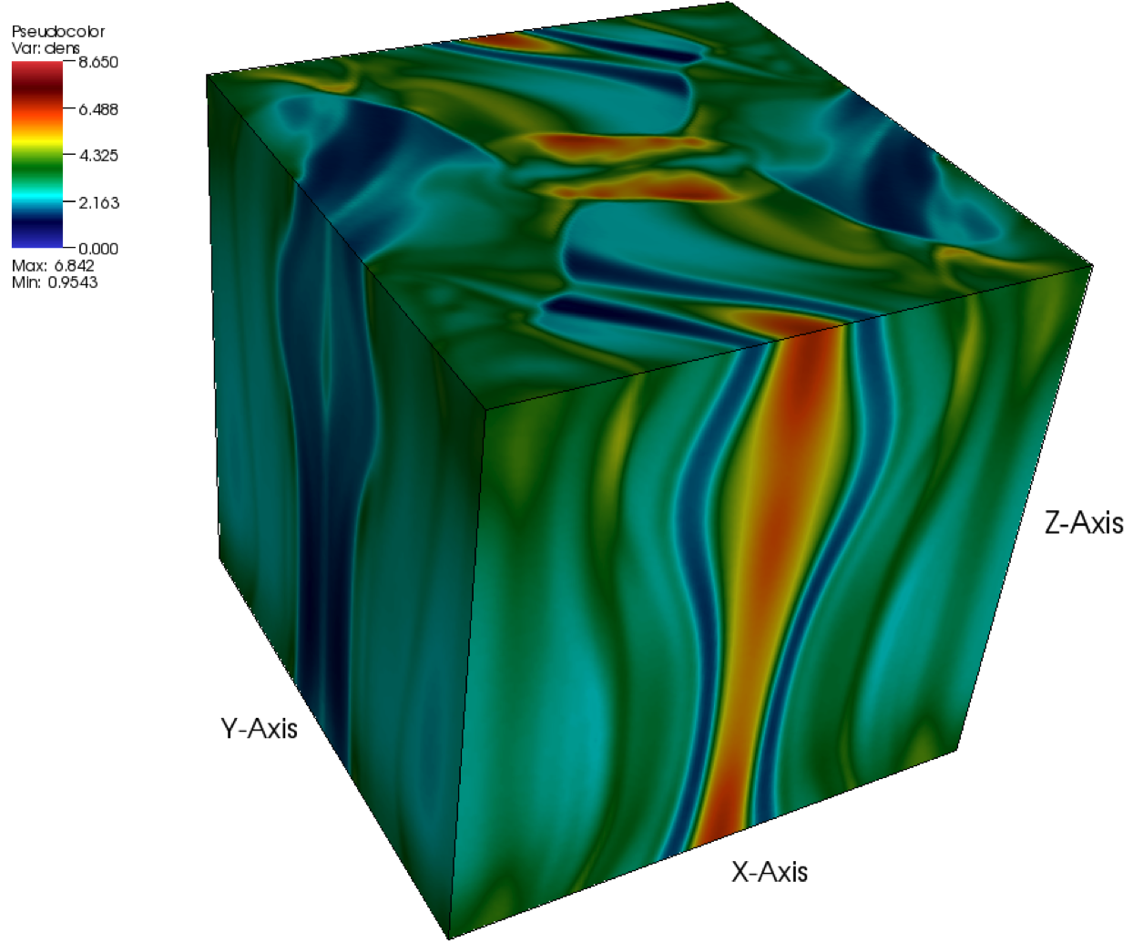 [c]
[c] 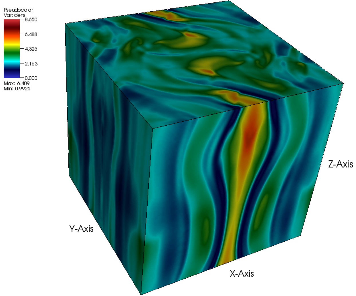 [d]
[d] 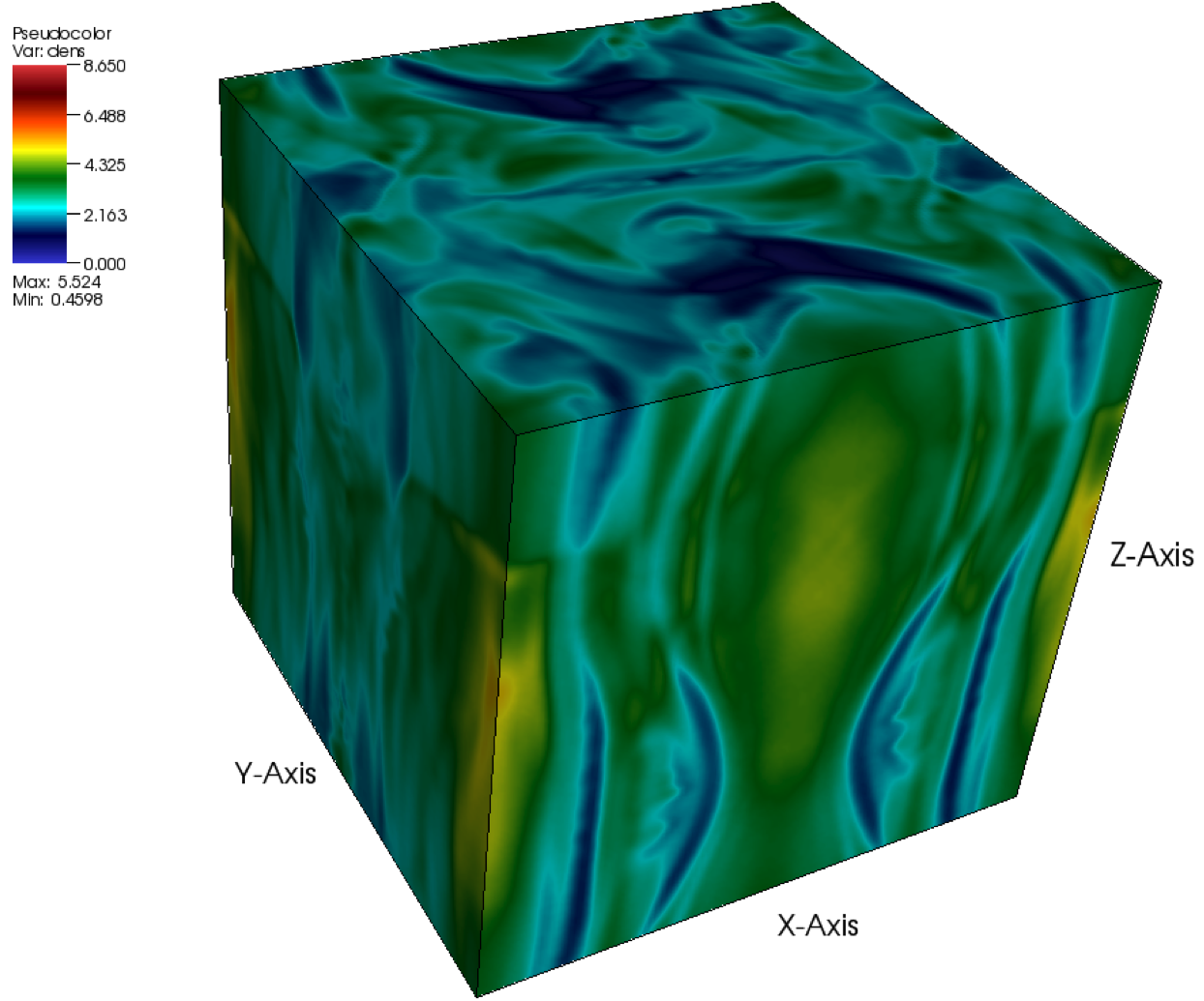
|
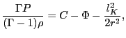
The magnetized accretion torus problem is based on the global magneto-rotational instability (MRI)
simulations of Hawley (2000). It can be found under magnetoHD/Torus.
We consider a magnetized torus of constant angular
momentum (
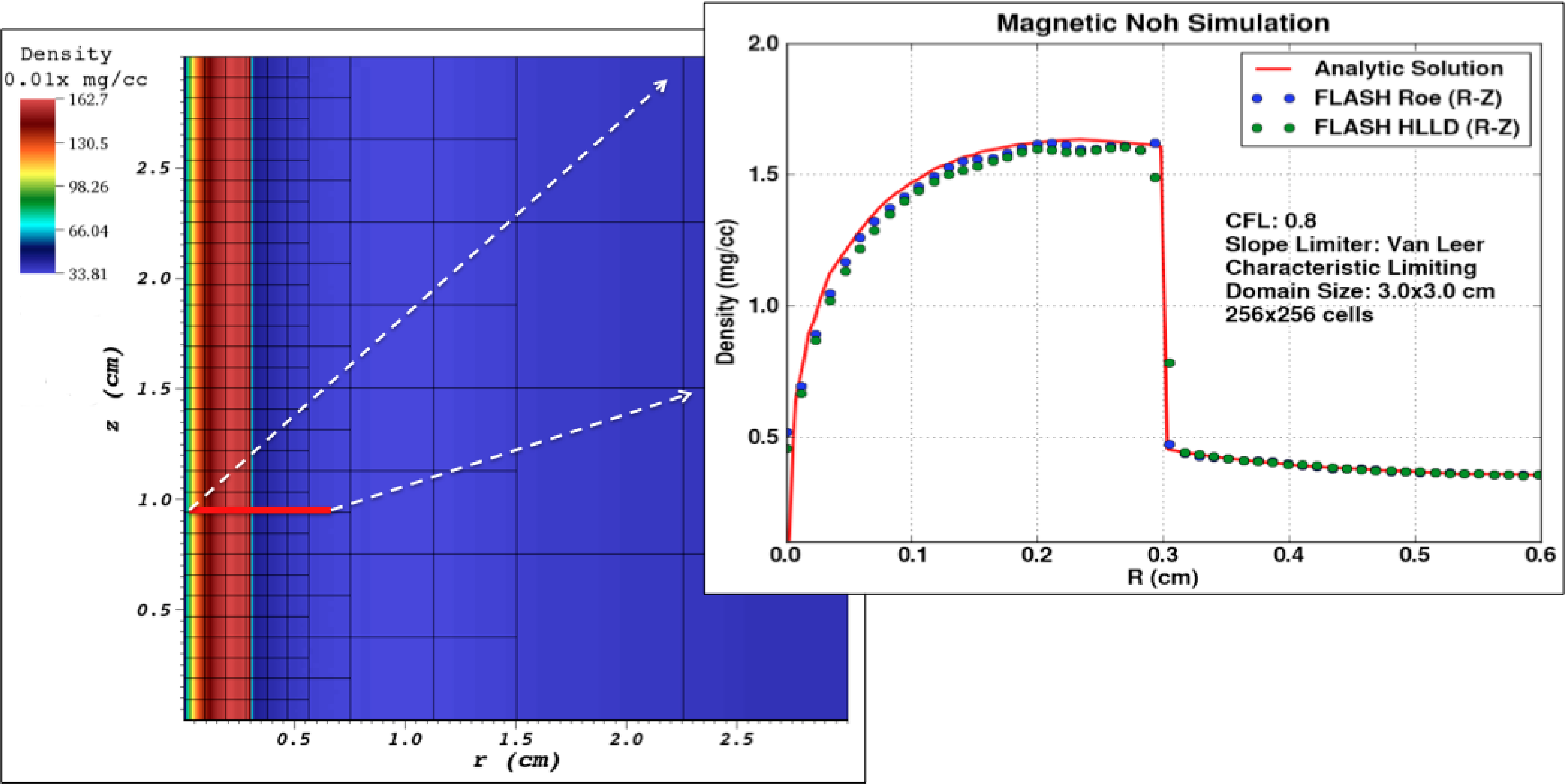
![]() ), inside a normalized Paczynsky-Wiita pseudo-Newtonean
gravitational potential (Paczynsky&Wiita, 1980) of the form
), inside a normalized Paczynsky-Wiita pseudo-Newtonean
gravitational potential (Paczynsky&Wiita, 1980) of the form
![]() , where
, where
![]() .
.
The cylindrical computational domain, with lengths normalized at ![]() ,
extends from 1.5
,
extends from 1.5 ![]() to 15.5
to 15.5 ![]() in the radial direction and from -7
in the radial direction and from -7 ![]() to 7
to 7 ![]() in the
in the ![]() direction. For this specific simulation we use seven levels of
refinement, linear reconstruction with vanLeer limiter and the HLLC Riemann solver.
The boundary conditions are set to outflow, except for
the leftmost side where a diode-like condition is applied.
direction. For this specific simulation we use seven levels of
refinement, linear reconstruction with vanLeer limiter and the HLLC Riemann solver.
The boundary conditions are set to outflow, except for
the leftmost side where a diode-like condition is applied.
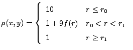
Assuming an adiabatic equation of state, the initial density profile of the torus is given by
 |
(35.18) |
We allow the system to evolve for
![]() . The torus is MRI unstable and
after approximately one revolution accretion sets in. The strong shear generates
an azimuthal field component and the angular momentum is redistributed.
Due to the instability, fillamentary structures form at the torus surface
that account for its rich morphology (Figure 35.49).
These results can be promtly compared to those in Hawley (2000) and
Mignone et al. (2007).
. The torus is MRI unstable and
after approximately one revolution accretion sets in. The strong shear generates
an azimuthal field component and the angular momentum is redistributed.
Due to the instability, fillamentary structures form at the torus surface
that account for its rich morphology (Figure 35.49).
These results can be promtly compared to those in Hawley (2000) and
Mignone et al. (2007).
|
In this test we consider the magnetized version of the classical Noh problem (Noh, 1987). It consists of a cylindrically symmetric implosion of a pressure-less gas: the gas stagnates at the symmetry axis and creates an outward moving accretion shock which propagates at a constant velocity. The self-similar analytic solution of this problem has been widely used as benchmark test for hydrodynamic codes, especially those targeting implosion.
Recently, Velikovich et al. (2012) have extended the original test problem to include an embedded azimuthal magnetic field, in accordance with the Z-pinch physics. In their study, they present a family of exact analytic solutions for which the values of primitive variables are finite everywhere, providing an excellent benchmark for Z-pinch and general MHD codes.
We perform this test in both cartesian and cylindrical geometries. The tests can be found respectively in magnetoHD/Noh and magnetoHD/NohCylindrical. For brevity we describe only the cylindrical initialization. The cartesian can be easily recovered by projecting the solution onto the X-Y plane. A 3T MHD version of this test can also be found under magnetoHD/unitTest/NohCylindricalRagelike.
The simulation is initialized in a computational box that spans ![]() cm in the
cm in the
![]() and
and ![]() directions, in cylindrical (
directions, in cylindrical (![]() ) geometry. The leftmost boundary condition
is set to axisymmetry, whereas the remaining boundaries are set to outflow (zero gradient).
The initial condition in primitive variables is defined as
) geometry. The leftmost boundary condition
is set to axisymmetry, whereas the remaining boundaries are set to outflow (zero gradient).
The initial condition in primitive variables is defined as
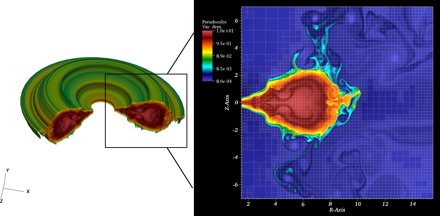
The simulations are evolved for ![]() ns, utilizing the unsplit solver
and a Courant number of 0.8. We use 6 levels
of refinement, corresponding to an equivalent resolution of
ns, utilizing the unsplit solver
and a Courant number of 0.8. We use 6 levels
of refinement, corresponding to an equivalent resolution of
![]() zones. The
reconstruction is piecewise-linear (second order) with characteristic limiting,
whereas the Riemann solvers employed are the HLLD and Roe.
zones. The
reconstruction is piecewise-linear (second order) with characteristic limiting,
whereas the Riemann solvers employed are the HLLD and Roe.
The resulting density profile is shown in Figure 35.50. The refinement
closely follows the propagation of the discontinuity which reaches
the analytically predicted location (![]() cm) at
cm) at ![]() ns. The lineouts for HLLD (green dots)
and Roe (blue dots) shown on the right, display good agreement with the analytic solution
(red line) and the discontinuity is sharply captured (resolved on two points).
Our Figure 35.50 can be directly compared to Figures 2a and 3a of Velikovich et al. (2012).
ns. The lineouts for HLLD (green dots)
and Roe (blue dots) shown on the right, display good agreement with the analytic solution
(red line) and the discontinuity is sharply captured (resolved on two points).
Our Figure 35.50 can be directly compared to Figures 2a and 3a of Velikovich et al. (2012).
|
 |
(35.20) |
 |
(35.21) |
 |
(35.22) |
| (35.23) | |||
| (35.24) | |||
| (35.25) |
|
[a] 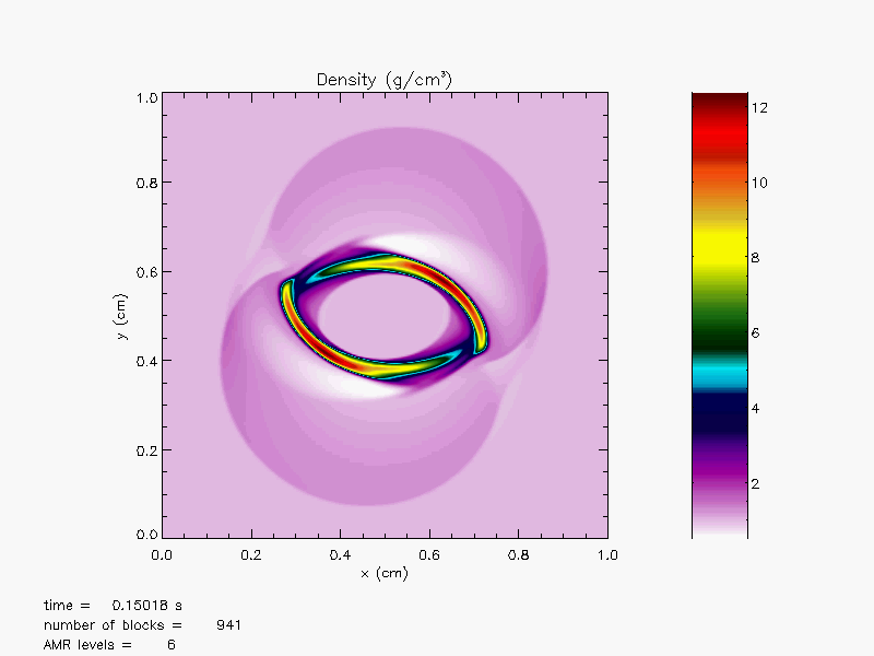 [b]
[b] 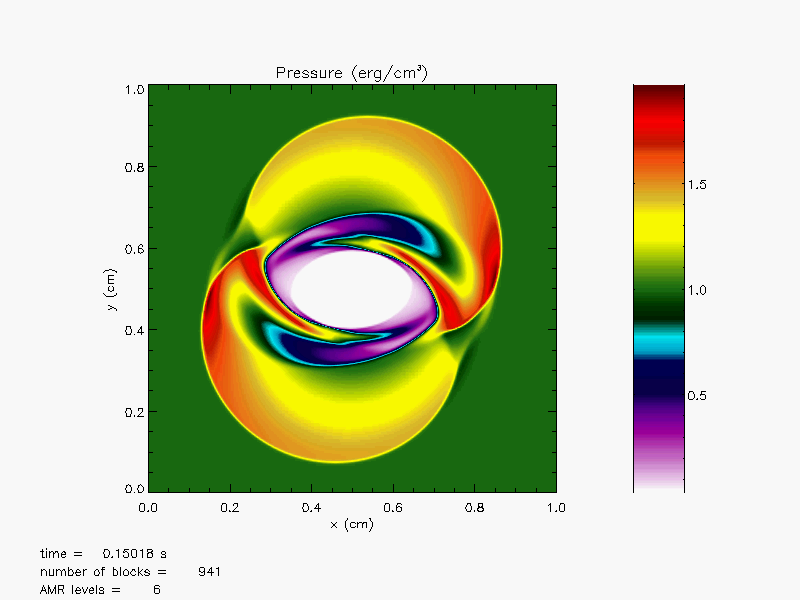 [c]
[c] 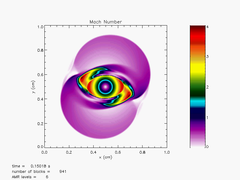 [d]
[d] 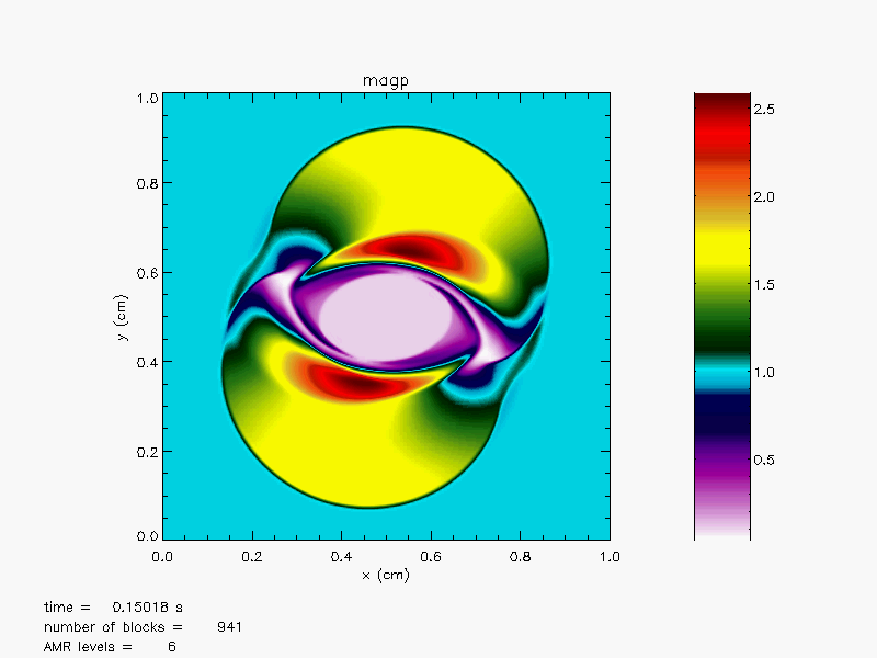
|
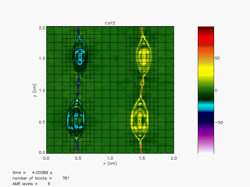
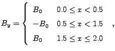
The two-dimensional current sheet problem, magnetoHD/CurrentSheet, has recently been studied by Gardiner and Stone (2005) in ideal MHD regime. The two current sheets are initialized and therefore magnetic reconnections are inevitably driven. In the regions the magnetic reconnection takes place the magnetic flux approaches vanishingly small values, and the loss in the magnetic energy is converted into heat (thermal energy). This phenomenon changes the overall topology of the magnetic fields and hence affects the global magnetic configuration.
The square computational domain is given as
![]() with periodic
boundary conditions on all four sides.
We initialize two current sheets in the following:
with periodic
boundary conditions on all four sides.
We initialize two current sheets in the following:
 |
(35.26) |
The changes of the magnetic fields seed the magnetic reconnection and develop formations of magnetic islands along the two current sheets. The small islands are then merged into the bigger islands by continuously shifting up and down along the current sheets until there is one big island left in each current sheet.
The temporal evolution of the magnetic field lines from ![]() to
to ![]() are
shown in Figure 35.53(a) - Figure 35.53(f)
on a
are
shown in Figure 35.53(a) - Figure 35.53(f)
on a
![]() uniform grid.
In Figure 35.54 the same problem
is resolved on an AMR grid with 6 refinement levels, showing
the current density
uniform grid.
In Figure 35.54 the same problem
is resolved on an AMR grid with 6 refinement levels, showing
the current density ![]() along with the AMR block structures at
along with the AMR block structures at ![]() .
The StaggeredMesh solver was used for this problem.
.
The StaggeredMesh solver was used for this problem.
|
[a]  [b]
[b]  [c]
[c] 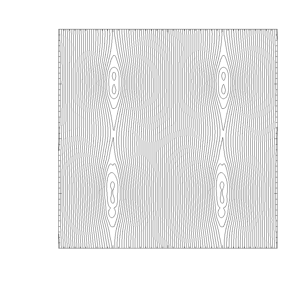 [d]
[d] 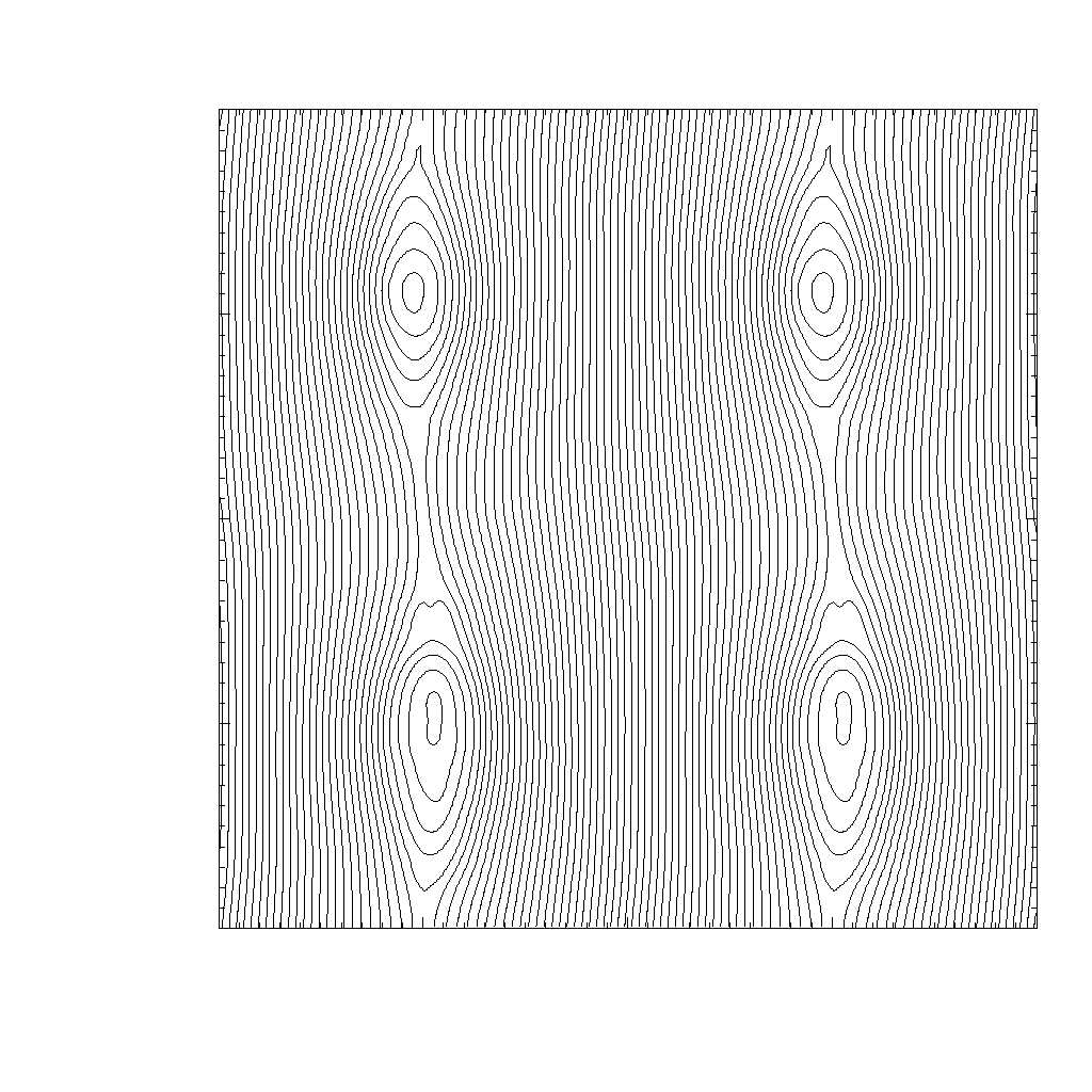 [e]
[e] 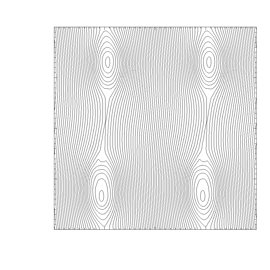 [f]
[f] 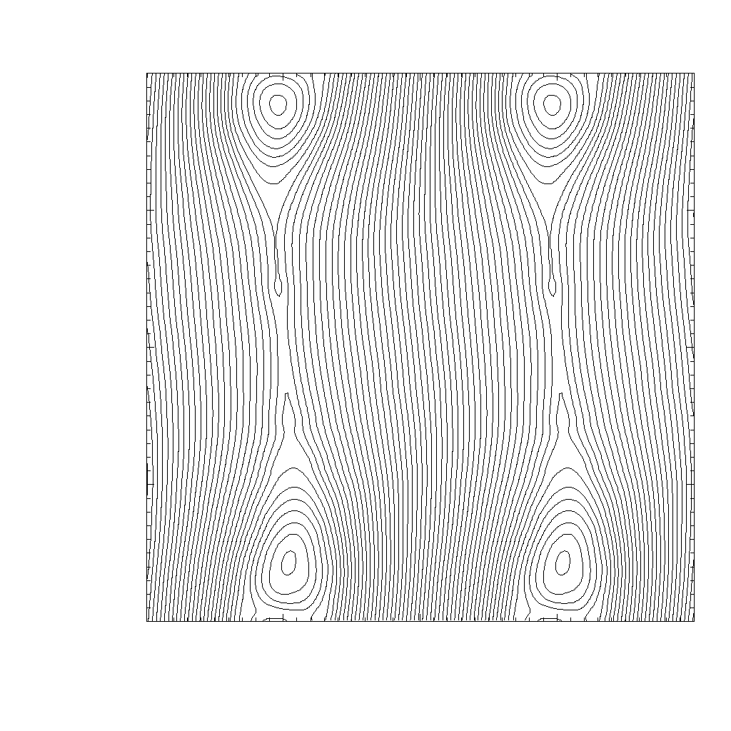
|
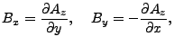
The computational domain is
![]() , with a grid resolution
, with a grid resolution
![]() , and doubly-periodic boundary conditions.
With this rectangular grid cell, the flow is not symmetric in
, and doubly-periodic boundary conditions.
With this rectangular grid cell, the flow is not symmetric in ![]() and
and ![]() directions because the field loop does not advect across each grid cell diagonally and hence the resulting fluxes are different in
directions because the field loop does not advect across each grid cell diagonally and hence the resulting fluxes are different in ![]() and
and ![]() directions.
The density and pressure are unity everywhere and
directions.
The density and pressure are unity everywhere and
![]() . The velocity fields are defined as,
. The velocity fields are defined as,
 |
(35.28) |
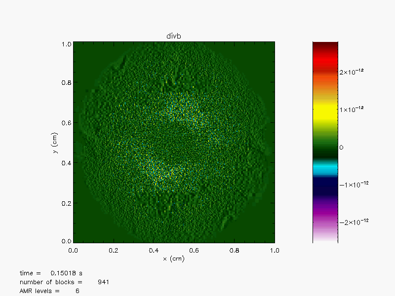
By using this initialization process, divergence-free magnetic fields are constructed with a maximum value of
![]() in the order of
in the order of ![]() at the chosen resolution. The parameters in (35.29) are
at the chosen resolution. The parameters in (35.29) are
![]() and a field loop radius
and a field loop radius ![]() . This initial condition results in a very high plasma beta
. This initial condition results in a very high plasma beta
![]() for the inner region of the field loop. Inside the loop the magnetic field strength is very weak and the flow dynamics is dominated by the gas pressure.
for the inner region of the field loop. Inside the loop the magnetic field strength is very weak and the flow dynamics is dominated by the gas pressure.
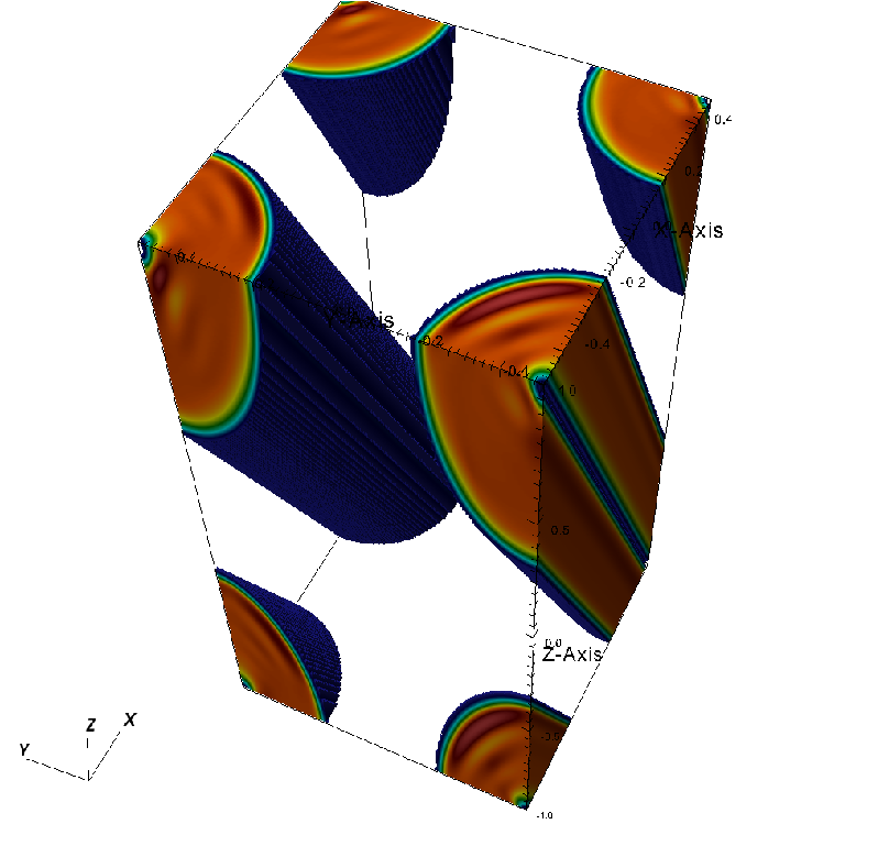
The field loop advection is integrated to a final time ![]() . The
advection test is found to truly require the full multidimensional MHD
approach (Gardiner and Stone, 2005, 2008; Lee and Deane, 2008). Since
the field loop is advected at an oblique angle to the
. The
advection test is found to truly require the full multidimensional MHD
approach (Gardiner and Stone, 2005, 2008; Lee and Deane, 2008). Since
the field loop is advected at an oblique angle to the ![]() -axis of the
computational domain, the values of
-axis of the
computational domain, the values of
![]() and
and
![]() are non-zero in general and their roles are
crucial in multidimensional MHD flows.
These terms, together with the multidimensional MHD terms
are non-zero in general and their roles are
crucial in multidimensional MHD flows.
These terms, together with the multidimensional MHD terms
![]() and
and
![]() , are explicitly included in the data
reconstruction-evolution algorithm in the USM scheme (see Lee and Deane, 2008).
During the advection a good
numerical scheme should maintain: (a) the circular symmetry of the
loop at all time: a numerical scheme that lacks proper numerical
dissipation results in spurious oscillations at the loop, breaking the
circular symmetry; (b)
, are explicitly included in the data
reconstruction-evolution algorithm in the USM scheme (see Lee and Deane, 2008).
During the advection a good
numerical scheme should maintain: (a) the circular symmetry of the
loop at all time: a numerical scheme that lacks proper numerical
dissipation results in spurious oscillations at the loop, breaking the
circular symmetry; (b) ![]() during the simulation:
during the simulation: ![]() will grow
proportional to
will grow
proportional to
![]() if a numerical
scheme does not properly include multidimensional MHD terms.
if a numerical
scheme does not properly include multidimensional MHD terms.
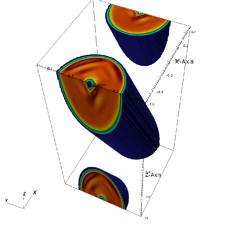
From the results in Figure 35.55, the USM scheme maintains the circular shape of the loop extremely well to the final time step. The scheme successfully retains the initial circular symmetry and does not develop severe oscillations.
|
[a] 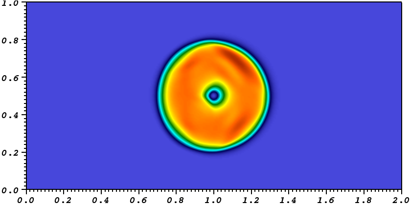 [b]
[b]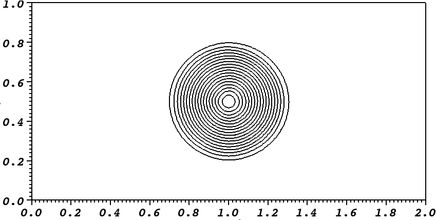
|
A variant 3D version of this problem (Gardiner and Stone, 2008) is also available, and is illustrated in in Fig. 35.56. This problem is considered to be a particularly challenging test because the correct solution requires inclusion of the multidimensional MHD terms to preserve the in-plane dynamics. Otherwise, the failure in preserving the in-plane dynamics (i.e., growth in the out-of-plane component) results in erroneous behavior of the field loop. As shown in Fig. 35.56, the USM solver successfully maintains the circular shape of the field loop and maintains the out-of-plane component of the magnetic field to very small values over the domain. This figure compares very well with Fig. 2 in Gardiner and Stone, 2008.
|
[  [
[ [
[
|
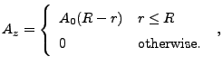
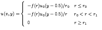
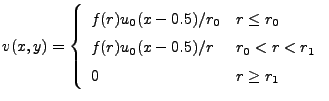
This problem can be computed in various magnetized flow regimes by considering
different magnetic field strengths. The computational domain is a square
![]() with a maximum refinement level 4. The explosion is driven by an over-pressurized circular region at the center of the domain with a radius
with a maximum refinement level 4. The explosion is driven by an over-pressurized circular region at the center of the domain with a radius ![]() . The initial density is unity everywhere, and the pressure of the ambient gas is
. The initial density is unity everywhere, and the pressure of the ambient gas is ![]() , whereas
the pressure of the inner region is
, whereas
the pressure of the inner region is ![]() . The strength of a uniform magnetic field in the
. The strength of a uniform magnetic field in the ![]() -direction are 0,
-direction are 0,
![]() and
and
![]() . This initial condition results in a very low-
. This initial condition results in a very low-![]() ambient plasma state,
ambient plasma state,
![]() . Through this low-
. Through this low-![]() ambient state, the explosion emits almost spherical fast magneto-sonic shocks that propagate with the fastest wave speed. The flow has
ambient state, the explosion emits almost spherical fast magneto-sonic shocks that propagate with the fastest wave speed. The flow has
![]() .
.
With this strong magnetic field strength,
![]() , shown in Figure 35.57, the explosion now becomes highly anisotropic as shown in the pressure plot in Figure 35.57. The Figure shows that the displacement of gas in the transverse
, shown in Figure 35.57, the explosion now becomes highly anisotropic as shown in the pressure plot in Figure 35.57. The Figure shows that the displacement of gas in the transverse ![]() -direction is increasingly inhibited and hydrodynamical shocks propagate in both positive and negative
-direction is increasingly inhibited and hydrodynamical shocks propagate in both positive and negative ![]() -directions parallel to
-directions parallel to ![]() . This process continues until total pressure equilibrium is reached in the central region.
This problem is also available in 2D setup.
. This process continues until total pressure equilibrium is reached in the central region.
This problem is also available in 2D setup.
|
[a] 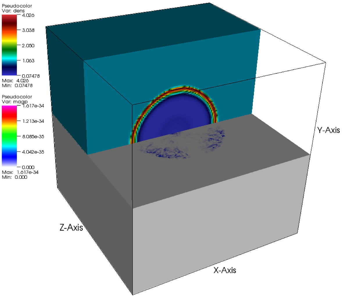 [b]
[b] 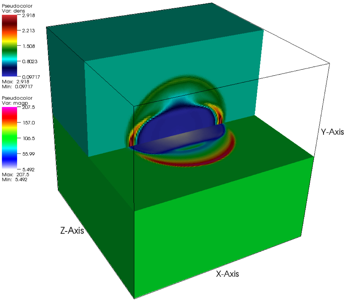 [c]
[c] 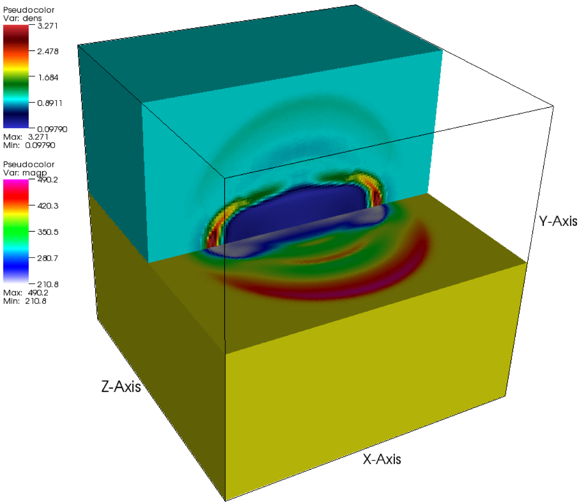
|