Next: 35.2 Magnetohydrodynamics Test Problems Up: 35. The Supplied Test Previous: 35. The Supplied Test Contents Index
The Sod problem (Sod 1978) is a one-dimensional flow discontinuity problem that provides a good test of a compressible code's ability to capture shocks and contact discontinuities with a small number of cells and to produce the correct profile in a rarefaction. It also tests a code's ability to correctly satisfy the Rankine-Hugoniot shock jump conditions. When implemented at an angle to a multidimensional grid, it can be used to detect irregularities in planar discontinuities produced by grid geometry or operator splitting effects.
We construct the initial conditions for the Sod problem by establishing a
planar interface at some angle to the ![]() - and
- and ![]() -axes. The fluid is initially
at rest on either side of the interface, and the density and pressure jumps
are chosen so that all three types of nonlinear, hydrodynamic waves
(shock, contact, and rarefaction) develop.
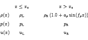
To the “left” and “right” of the interface we have
-axes. The fluid is initially
at rest on either side of the interface, and the density and pressure jumps
are chosen so that all three types of nonlinear, hydrodynamic waves
(shock, contact, and rarefaction) develop.
To the “left” and “right” of the interface we have
 |
(35.1) |
In FLASH, the Sod problem (Sod) uses the runtime parameters
listed in Table 35.1 in addition to those supplied
by default with the code. For this problem we use the Gamma equation of
state alternative implementation and set gamma to 1.4. The default values listed
in Table 35.1 are appropriate to a shock with
normal parallel to the ![]() -axis that initially intersects that axis
at
-axis that initially intersects that axis
at ![]() (halfway across a box with unit dimensions).
(halfway across a box with unit dimensions).
| Variable | Type | Default | Description |
| sim_rhoLeft | real | 1 | Initial density to the
left of the interface
(
|
| sim_rhoRight | real | 0.125 | Initial density to the
right (
|
| sim_pLeft | real | 1 | Initial pressure to the
left ( |
| sim_pRight | real | 0.1 | Initial pressure to the
right ( |
| sim_uLeft | real | 0 | Initial velocity
(perpendicular to interface)
to the left ( |
| sim_uRight | real | 0 | Initial velocity
(perpendicular to interface)
to the right ( |
| sim_xangle | real | 0 | Angle made by interface
normal with the |
| sim_yangle | real | 90 | Angle made by interface
normal with the |
| sim_posn | real | 0.5 | Point of intersection between
the interface plane and the
|
|
|
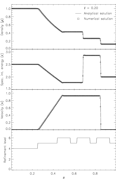
Figure 35.2 shows the result of running the Sod problem
with FLASH on a two-dimensional grid with the analytical solution
shown for comparison. The hydrodynamical algorithm used here is the
directionally split piecewise-parabolic method (PPM) included with
FLASH. In this run the shock normal is chosen to be parallel to the
![]() -axis. With six levels of refinement, the effective grid size at
the finest level is
-axis. With six levels of refinement, the effective grid size at
the finest level is ![]() , so the finest cells have width
0.00390625. At
, so the finest cells have width
0.00390625. At ![]() , three different nonlinear waves are present:
a rarefaction between
, three different nonlinear waves are present:
a rarefaction between ![]() and
and ![]() , a contact
discontinuity at
, a contact
discontinuity at ![]() , and a shock at
, and a shock at ![]() . The two
discontinuities are resolved with approximately two to three cells
each at the highest level of refinement, demonstrating the ability
of PPM to handle sharp flow features well. Near the contact
discontinuity and in the rarefaction, we find small errors of about
. The two
discontinuities are resolved with approximately two to three cells
each at the highest level of refinement, demonstrating the ability
of PPM to handle sharp flow features well. Near the contact
discontinuity and in the rarefaction, we find small errors of about
![]() in the density and specific internal energy, with similar
errors in the velocity inside the rarefaction. Elsewhere, the
numerical solution is close to exact; no oscillations are present.
in the density and specific internal energy, with similar
errors in the velocity inside the rarefaction. Elsewhere, the
numerical solution is close to exact; no oscillations are present.
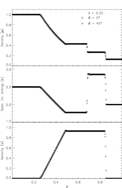
Figure 35.3 shows the result of running the Sod
problem on the same two-dimensional grid with different shock
normals: parallel to the ![]() -axis (
-axis (
![]() ) and along the
box diagonal (
) and along the
box diagonal (
![]() ). For the diagonal solution, we have
interpolated values of density, specific internal energy, and
velocity to a set of 256 points spaced exactly as in the
). For the diagonal solution, we have
interpolated values of density, specific internal energy, and
velocity to a set of 256 points spaced exactly as in the ![]() -axis
solution. This comparison shows the effects of the second-order
directional splitting used with FLASH on the resolution of shocks.
At the right side of the rarefaction and at the contact
discontinuity, the diagonal solution undergoes slightly larger
oscillations (on the order of a few percent) than the
-axis
solution. This comparison shows the effects of the second-order
directional splitting used with FLASH on the resolution of shocks.
At the right side of the rarefaction and at the contact
discontinuity, the diagonal solution undergoes slightly larger
oscillations (on the order of a few percent) than the ![]() -axis
solution. Also, the value of each variable inside the discontinuity
regions differs between the two solutions by up to 10%. However,
the location and thickness of the discontinuities is the same for
the two solutions. In general, shocks at an angle to the grid are
resolved with approximately the same number of cells as shocks
parallel to a coordinate axis.
-axis
solution. Also, the value of each variable inside the discontinuity
regions differs between the two solutions by up to 10%. However,
the location and thickness of the discontinuities is the same for
the two solutions. In general, shocks at an angle to the grid are
resolved with approximately the same number of cells as shocks
parallel to a coordinate axis.
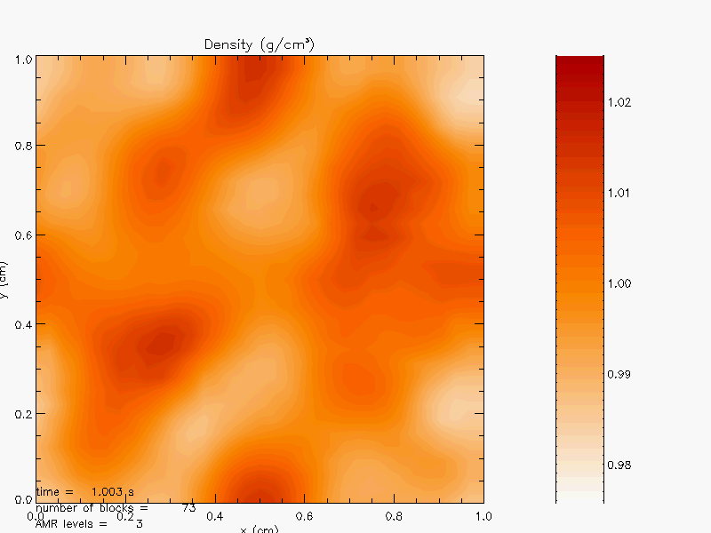
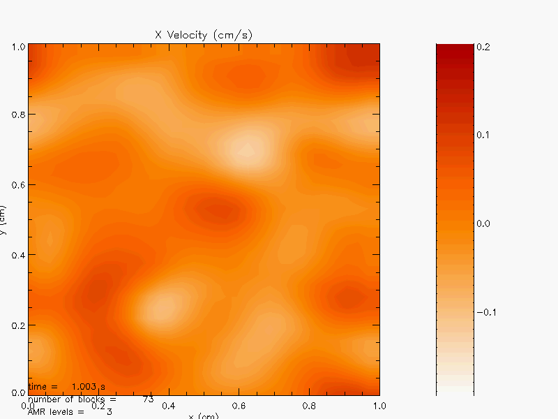
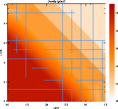
Figure 35.4 presents a colormap plot of the density at
![]() in the diagonal solution together with the block structure
of the AMR grid. Note that regions surrounding the discontinuities
are maximally refined, while behind the shock and contact
discontinuity, the grid has de-refined, because the second
derivative of the density has decreased in magnitude. Because
zero-gradient outflow boundaries were used for this test, some
reflections are present at the upper left and lower right corners,
but at
in the diagonal solution together with the block structure
of the AMR grid. Note that regions surrounding the discontinuities
are maximally refined, while behind the shock and contact
discontinuity, the grid has de-refined, because the second
derivative of the density has decreased in magnitude. Because
zero-gradient outflow boundaries were used for this test, some
reflections are present at the upper left and lower right corners,
but at ![]() these have not yet propagated to the center of the
grid.
these have not yet propagated to the center of the
grid.
|
This Blast2 problem was originally used by Woodward and Colella (1984) to compare the performance of several different hydrodynamical methods on problems involving strong shocks and narrow features. It has no analytical solution (except at very early times), but since it is one-dimensional, it is easy to produce a converged solution by running the code with a very large number of cells, permitting an estimate of the self-convergence rate. For FLASH, it also provides a good test of the adaptive mesh refinement scheme.
The initial conditions consist of two parallel, planar flow discontinuities. Reflecting boundary conditions are used. The density is unity and the velocity is zero everywhere. The pressure is large at the left and right and small in the center
| (35.2) |
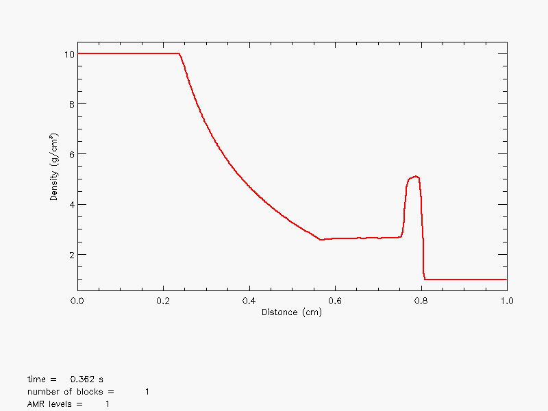
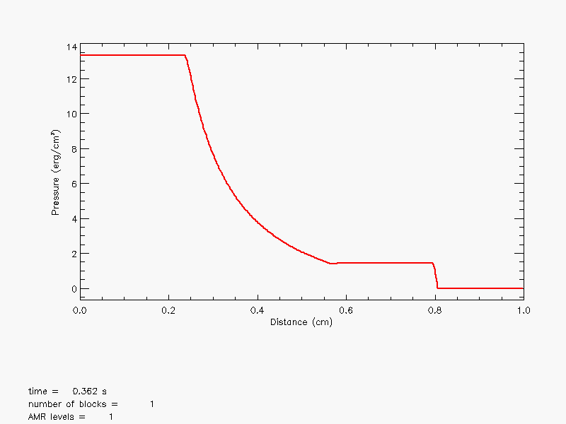
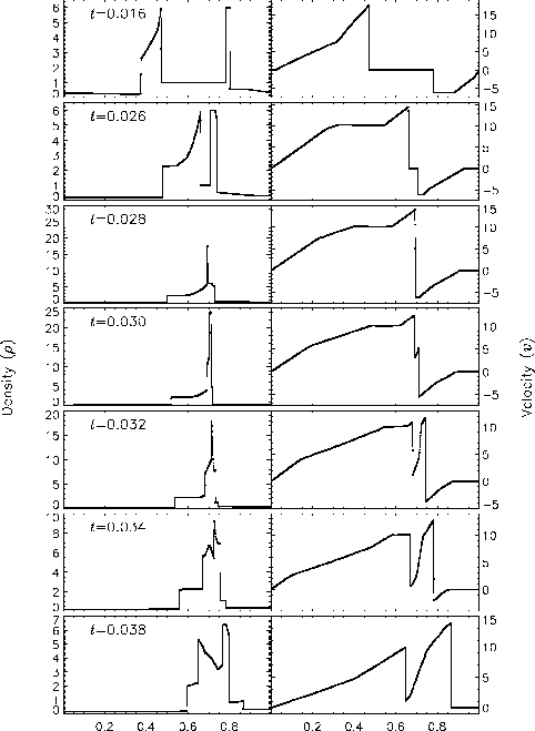
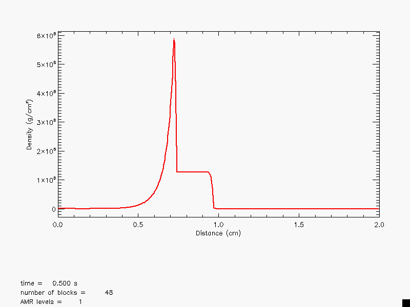
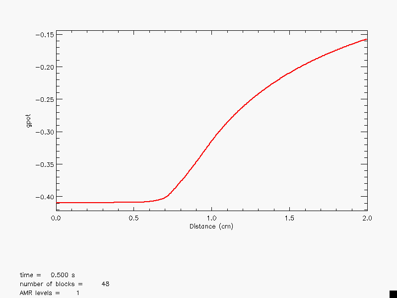
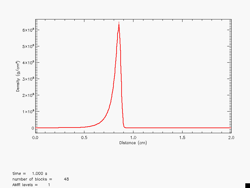
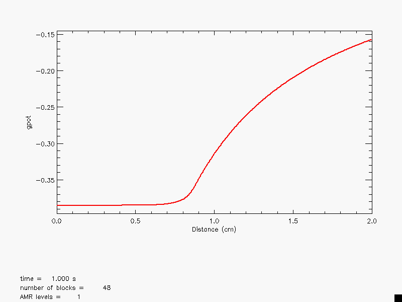
Figure 35.5 shows the density and velocity profiles at
several different times in the converged solution, demonstrating the
complexity inherent in this problem. The initial pressure
discontinuities drive shocks into the middle part of the grid;
behind them, rarefactions form and propagate toward the outer
boundaries, where they are reflected back into the grid. By the time
the shocks collide at ![]() , the reflected rarefactions have
caught up to them, weakening them and making their post-shock
structure more complex. Because the right-hand shock is initially
weaker, the rarefaction on that side reflects from the wall later,
so the resulting shock structures going into the collision from the
left and right are quite different. Behind each shock is a contact
discontinuity left over from the initial conditions (at
, the reflected rarefactions have
caught up to them, weakening them and making their post-shock
structure more complex. Because the right-hand shock is initially
weaker, the rarefaction on that side reflects from the wall later,
so the resulting shock structures going into the collision from the
left and right are quite different. Behind each shock is a contact
discontinuity left over from the initial conditions (at
![]() and 0.73). The shock collision produces an extremely high and
narrow density peak. The peak density should be slightly less than
30. However, the peak density shown in Figure 35.5 is
only about 18, since the maximum value of the density does not occur
at exactly
and 0.73). The shock collision produces an extremely high and
narrow density peak. The peak density should be slightly less than
30. However, the peak density shown in Figure 35.5 is
only about 18, since the maximum value of the density does not occur
at exactly ![]() . Reflected shocks travel back into the
colliding material, leaving a complex series of contact
discontinuities and rarefactions between them. A new contact
discontinuity has formed at the point of the collision (
. Reflected shocks travel back into the
colliding material, leaving a complex series of contact
discontinuities and rarefactions between them. A new contact
discontinuity has formed at the point of the collision (
![]() ). By
). By ![]() , the right-hand reflected shock has met the
original right-hand contact discontinuity, producing a strong
rarefaction, which meets the central contact discontinuity at
, the right-hand reflected shock has met the
original right-hand contact discontinuity, producing a strong
rarefaction, which meets the central contact discontinuity at
![]() . Between
. Between ![]() and
and ![]() , the slope of the density
behind the left-hand shock changes as the shock moves into a region
of constant entropy near the left-hand contact discontinuity.
, the slope of the density
behind the left-hand shock changes as the shock moves into a region
of constant entropy near the left-hand contact discontinuity.
|
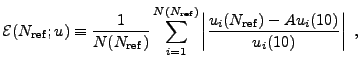
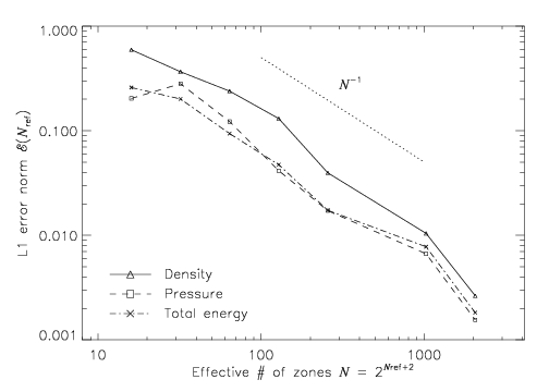
Figure 35.6 shows the self-convergence of density
and pressure when FLASH is run on this problem. We compare the
density, pressure, and total specific energy at ![]() obtained
using FLASH with ten levels of refinement to solutions using several
different maximum refinement levels. This figure plots the L1 error
norm for each variable
obtained
using FLASH with ten levels of refinement to solutions using several
different maximum refinement levels. This figure plots the L1 error
norm for each variable ![]() , defined using
, defined using
Although PPM is formally a second-order method, the convergence rate is only linear. This is not surprising, since the order of accuracy of a method applies only to smooth flow and not to flows containing discontinuities. In fact, all shock capturing schemes are only first-order accurate in the vicinity of discontinuities. Indeed, in their comparison of the performance of seven nominally second-order hydrodynamic methods on this problem, Woodward and Colella found that only PPM achieved even linear convergence; the other methods were worse. The error norm is very sensitive to the correct position and shape of the strong, narrow shocks generated in this problem.
The additional runtime parameters supplied with the 2blast
problem are listed in Table 35.2. This problem is
configured to use the perfect-gas equation of state (gamma)
with gamma set to 1.4 and is run in a two-dimensional unit
box. Boundary conditions in the ![]() -direction (transverse to the
shock normals) are taken to be periodic.
-direction (transverse to the
shock normals) are taken to be periodic.
|
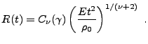
The Sedov explosion problem (Sedov 1959) is another purely hydrodynamical test in which we check the code's ability to deal with strong shocks and non-planar symmetry. The problem involves the self-similar evolution of a cylindrical or spherical blast wave from a delta-function initial pressure perturbation in an otherwise homogeneous medium. We provide two different ways to generate the initial conditions:
 |
(35.4) |
We set the ratio of specific heats
![]() .
In running this problem we choose
.
In running this problem we choose ![]() to be 3.5
times as large as the finest adaptive mesh resolution in order to minimize
effects due to the Cartesian geometry of our grid.
The density
is set equal to
to be 3.5
times as large as the finest adaptive mesh resolution in order to minimize
effects due to the Cartesian geometry of our grid.
The density
is set equal to ![]() everywhere, and the
pressure is set to a small value
everywhere, and the
pressure is set to a small value
![]() everywhere but in the center
of the grid.
The fluid is initially at rest.
In the self-similar blast wave that develops for
everywhere but in the center
of the grid.
The fluid is initially at rest.
In the self-similar blast wave that develops for ![]() , the
density, pressure, and radial velocity are all functions of
, the
density, pressure, and radial velocity are all functions of
![]() , where
, where
 |
(35.5) |
| (35.6) | |||
| (35.7) | |||
|
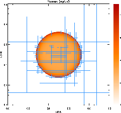
Figure 35.8 shows the pressure field in the
8-level calculation at ![]() together with the block refinement
pattern. Note that a relatively small fraction of the grid is
maximally refined in this problem. Although the pressure gradient at
the center of the grid is small, this region is refined because of
the large temperature gradient there. This illustrates the ability
of PARAMESH to refine grids using several different variables at
once.
together with the block refinement
pattern. Note that a relatively small fraction of the grid is
maximally refined in this problem. Although the pressure gradient at
the center of the grid is small, this region is refined because of
the large temperature gradient there. This illustrates the ability
of PARAMESH to refine grids using several different variables at
once.
|
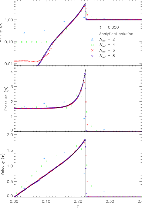
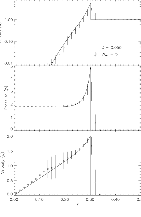
We have also run FLASH on the spherically symmetric Sedov problem in
order to verify the code's performance in three dimensions. The
results at ![]() using five levels of grid refinement are shown
in Figure 35.9. In this figure we have plotted the
average values as well as the root-mean-square (RMS) deviations from
the averages. As in the two-dimensional runs, the shock is spread
over about two cells at the finest AMR resolution in this run. The
width of the pressure peak in the analytical solution is about 1 1/2
cells at this time, so the maximum pressure is not captured in the
numerical solution. Behind the shock the numerical solution average
tracks the analytical solution quite well, although the Cartesian
grid geometry produces RMS deviations of up to 40% in the density
and velocity in the de-refined region well behind the shock. This
behavior is similar to that exhibited in the two-dimensional problem
at comparable resolution.
using five levels of grid refinement are shown
in Figure 35.9. In this figure we have plotted the
average values as well as the root-mean-square (RMS) deviations from
the averages. As in the two-dimensional runs, the shock is spread
over about two cells at the finest AMR resolution in this run. The
width of the pressure peak in the analytical solution is about 1 1/2
cells at this time, so the maximum pressure is not captured in the
numerical solution. Behind the shock the numerical solution average
tracks the analytical solution quite well, although the Cartesian
grid geometry produces RMS deviations of up to 40% in the density
and velocity in the de-refined region well behind the shock. This
behavior is similar to that exhibited in the two-dimensional problem
at comparable resolution.
|
The additional runtime parameters supplied with the Sedov problem are listed in Table 35.3. This problem is configured to use the perfect-gas equation of state (Gamma) with gamma set to 1.4. It is simulated in a unit-sized box.
| Variable | Type | Default | Description |
| sim_pAmbient | real | Initial ambient pressure
( |
|
| sim_rhoAmbient | real | 1 | Initial ambient density
( |
| sim_expEnergy | real | 1 | Explosion energy ( |
| sim_rInit | real | 0.05 | Radius of initial pressure
perturbation ( |
| sim_xctr | real | 0.5 | |
| sim_yctr | real | 0.5 | |
| sim_zctr | real | 0.5 | |
| sim_nSubZones | integer | 7 | Number of sub-cells in cells for applying the 1D profile |
 |
|
The two-dimensional isentropic vortex problem is often used as a benchmark for comparing numerical methods for fluid dynamics. The flow-field is smooth (there are no shocks or contact discontinuities) and contains no steep gradients, and the exact solution is known. It was studied by Yee, Vinokur, and Djomehri (2000) and by Shu (1998). In this subsection the problem is described, the FLASH control parameters are explained, and some results demonstrating how the problem can be used are presented.
The simulation domain is a square, and the center of the vortex is
located at
![]() . The flow-field is defined in
coordinates centered on the vortex center
. The flow-field is defined in
coordinates centered on the vortex center
![]() with
with
![]() . The domain is periodic, but
it is assumed that off-domain vortexes do not interact with the
primary; practically, this assumption can be
satisfied by ensuring that the simulation domain is large enough for a
particular vortex strength. We find that a domain size of
. The domain is periodic, but
it is assumed that off-domain vortexes do not interact with the
primary; practically, this assumption can be
satisfied by ensuring that the simulation domain is large enough for a
particular vortex strength. We find that a domain size of
![]() (specified through the Grid runtime parameters xmin,
xmax, ymin, and ymax) is sufficiently large for a
vortex strength (defined below) of 5.0. In the initialization below,
(specified through the Grid runtime parameters xmin,
xmax, ymin, and ymax) is sufficiently large for a
vortex strength (defined below) of 5.0. In the initialization below,
![]() and
and ![]() are the coordinates with respect to the nearest vortex
in the periodic sense.
are the coordinates with respect to the nearest vortex
in the periodic sense.
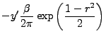
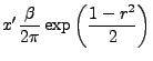
The ambient conditions are given by
![]() ,
, ![]() ,
,
![]() , and
, and ![]() , and the non-dimensional ambient temperature
is
, and the non-dimensional ambient temperature
is
![]() . Using the equation of state, the (dimensional)
. Using the equation of state, the (dimensional)
![]() is computed from
is computed from ![]() and
and
![]() . Perturbations are added to the velocity and
nondimensionalized temperature,
. Perturbations are added to the velocity and
nondimensionalized temperature,
![]() ,
,
![]() , and
, and
![]() according to
according to
| (35.11) | |||
 |
(35.12) |
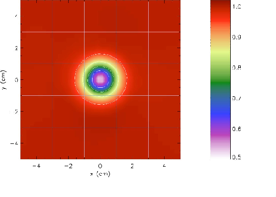
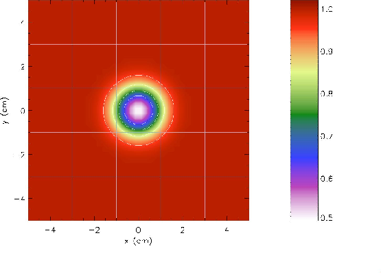
Figure 35.12 shows the exact density distribution represented on
a
![]() uniform grid with
uniform grid with
![]() . The
borders of each grid block (
. The
borders of each grid block (
![]() cells) are superimposed. In
addition to the shaded representation, contour lines are shown for
cells) are superimposed. In
addition to the shaded representation, contour lines are shown for
![]() , 0.85, 0.75, and 0.65. The density distribution is
radially symmetric, and the minimum density is
, 0.85, 0.75, and 0.65. The density distribution is
radially symmetric, and the minimum density is
![]() . Because the exact solution of the isentropic vortex
problem is the initial solution shifted by
. Because the exact solution of the isentropic vortex
problem is the initial solution shifted by
![]() , numerical phase (dispersion) and amplitude (dissipation) errors
are easy to identify. Dispersive errors distort the shape of the
vortex, breaking its symmetry. Dissipative errors smooth the
solution and flatten extrema; for the vortex, the minimum in density
at the vortex core will increase.
, numerical phase (dispersion) and amplitude (dissipation) errors
are easy to identify. Dispersive errors distort the shape of the
vortex, breaking its symmetry. Dissipative errors smooth the
solution and flatten extrema; for the vortex, the minimum in density
at the vortex core will increase.
|
A numerical simulation using the PPM scheme was run to illustrate
such errors. The simulation used the same grid shown in
Figure 35.12 with the same contour levels and color values. The
grid is intentionally coarse and the evolution time long to make
numerical errors visible. The vortex is represented by
approximately 8 grid points in each coordinate direction and is
advected diagonally with respect to the grid. At solution times of
![]() , etc., the vortex should be back at its initial
location.
, etc., the vortex should be back at its initial
location.
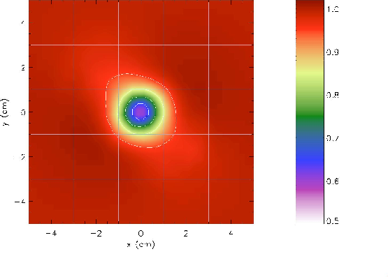
Figure 35.13 shows the solution at ![]() ; only slight
differences are observed. The density distribution is almost
radially symmetric, although the minimum density has risen to
; only slight
differences are observed. The density distribution is almost
radially symmetric, although the minimum density has risen to
![]() . Accumulating dispersion error is clearly visible at
. Accumulating dispersion error is clearly visible at
![]() (Figure 35.14), and the minimum density is now
(Figure 35.14), and the minimum density is now
![]() .
.
Figure 35.15 shows the density near ![]() at three simulation
times. The black line shows the initial condition. The red line
corresponds to
at three simulation
times. The black line shows the initial condition. The red line
corresponds to ![]() and the blue line to
and the blue line to ![]() . For the
later two times, the density is not radially symmetric. The lines
plotted are just representative profiles for those times, which give
an idea of the magnitude and character of the errors.
. For the
later two times, the density is not radially symmetric. The lines
plotted are just representative profiles for those times, which give
an idea of the magnitude and character of the errors.
|
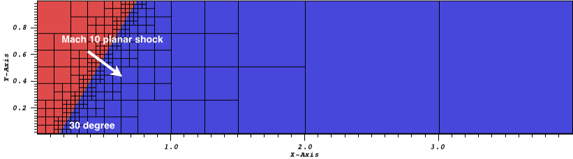
The initial setup involves a Mach 10 shock in air,
![]() , on a rectangular 2D domain of size
, on a rectangular 2D domain of size
![]() . The reflecting wall is represented as the bottom surface of the domain, beginning at
. The reflecting wall is represented as the bottom surface of the domain, beginning at ![]() .
The velocity normal to the incident shock in the post-shock region is 8.25, and the flow is at rest in the pre-shock region.
The undisturbed air ahead of the shock has a density of 1.4 and a pressure of 1.
See the initial density profile in Figure 35.16 resolved on 6 refinement AMR levels using 16
.
The velocity normal to the incident shock in the post-shock region is 8.25, and the flow is at rest in the pre-shock region.
The undisturbed air ahead of the shock has a density of 1.4 and a pressure of 1.
See the initial density profile in Figure 35.16 resolved on 6 refinement AMR levels using 16![]() -cell block size.
-cell block size.
The boundary condition on
![]() at
at ![]() is fixed in time with the initial values so that the reflected shock
is attached to the bottom surface. We impose reflecting boundary condition (i.e., negating the
is fixed in time with the initial values so that the reflected shock
is attached to the bottom surface. We impose reflecting boundary condition (i.e., negating the ![]() velocity field
velocity field ![]() )
on the rest of the bottom surface. On the top surface of
)
on the rest of the bottom surface. On the top surface of ![]() , we allow the initial Mach 10 shock proceeds
exactly as a function of time in order that the numerical evolution follows the oblique shock propagation without any planar distortion.
At
, we allow the initial Mach 10 shock proceeds
exactly as a function of time in order that the numerical evolution follows the oblique shock propagation without any planar distortion.
At ![]() , we impose a supersonic inflow boundary condition, and the outflow condition at
, we impose a supersonic inflow boundary condition, and the outflow condition at ![]() .
.
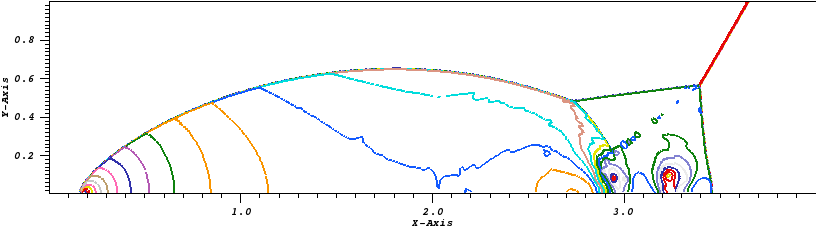
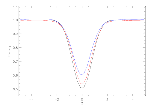
In later time, the solution develops to form two Mach stems and two contact discontinuities,
as shown in Figure 35.17 the density at ![]() sec. Also shown
in Figure 35.18 are 30 levels of contour lines of pressure,
illustrating the evolved flow discontinuities at
sec. Also shown
in Figure 35.18 are 30 levels of contour lines of pressure,
illustrating the evolved flow discontinuities at ![]() sec. We can also see that the numerical solution is
smooth and non-oscillatory in the region bounded by the curved reflected shock, the bottom surface and
the second Mach stem (see more discussion in Woodward and Colella, 1984).
sec. We can also see that the numerical solution is
smooth and non-oscillatory in the region bounded by the curved reflected shock, the bottom surface and
the second Mach stem (see more discussion in Woodward and Colella, 1984).
The 5th order WENO method in the unsplit hydrodynamics solver is used with a choice of hybrid Riemann solver which selectively adopts HLL only at strong shocks and HLLC otherwise.
|
| Variable | Type | Default | Description |
| sim_rhoLeft | real | 8 | Initial density to
the left of the shock
(
|
| sim_rhoRight | real | 1.4 | Initial density to the
right (
|
| sim_pLeft | real | 116.5 | Initial pressure to the
left ( |
| sim_pRight | real | 1 | Initial pressure to the
right ( |
| sim_uLeft | real | 7.1447096 | Initial |
| sim_uRight | real | 0 | Initial |
| sim_vLeft | real | -4.125 | Initial |
| sim_vRight | real | 0 | Initial |
| sim_xangle | real | -30 | Angle made by shock
normal with the |
| sim_yangle | real | 90 | Angle made by shock
normal with the |
| sim_posn | real | 1/6 | Point of intersection between
the shock plane and the
|
The problem uses a two-dimensional rectangular domain three units wide
and one unit high. Between ![]() and
and ![]() along the
along the ![]() -axis is a
step 0.2 units high. The step is treated as a reflecting boundary, as
are the lower and upper boundaries in the
-axis is a
step 0.2 units high. The step is treated as a reflecting boundary, as
are the lower and upper boundaries in the ![]() -direction. For the right-hand
-direction. For the right-hand
![]() -boundary, we use an outflow (zero gradient) boundary condition, while
on the left-hand side we use an inflow boundary. In the inflow boundary
cells, we set the density to
-boundary, we use an outflow (zero gradient) boundary condition, while
on the left-hand side we use an inflow boundary. In the inflow boundary
cells, we set the density to ![]() , the pressure to
, the pressure to ![]() , and the
velocity to
, and the
velocity to ![]() , with the latter directed parallel to the
, with the latter directed parallel to the ![]() -axis.
The domain itself is also initialized with these values.
We use
-axis.
The domain itself is also initialized with these values.
We use
| (35.13) |
|
The additional runtime parameters supplied with the
WindTunnel problem are listed in Table 35.6.
This problem is configured to use the perfect-gas
equation of state (Gamma) with gamma set to 1.4. We
also set
xmax![]() ,
ymax
,
ymax![]() ,
Nblockx
,
Nblockx![]() , and
Nblocky
, and
Nblocky![]() in order to create a grid with the correct
dimensions. The version of Simulation_defineDomain supplied with this
problem
removes all but the first three top-level blocks along the lower edge
of the grid to generate the step, and
gives REFLECTING boundaries to the obstacle blocks.
Finally, we
use xl_boundary_type = "user" (USER_DEFINED condition) and
xr_boundary_type = "outflow" (OUTFLOW boundary) to instruct FLASH to use
the correct boundary conditions in the
in order to create a grid with the correct
dimensions. The version of Simulation_defineDomain supplied with this
problem
removes all but the first three top-level blocks along the lower edge
of the grid to generate the step, and
gives REFLECTING boundaries to the obstacle blocks.
Finally, we
use xl_boundary_type = "user" (USER_DEFINED condition) and
xr_boundary_type = "outflow" (OUTFLOW boundary) to instruct FLASH to use
the correct boundary conditions in the ![]() -direction. Boundaries in
the
-direction. Boundaries in
the ![]() -direction are reflecting (REFLECTING).
-direction are reflecting (REFLECTING).
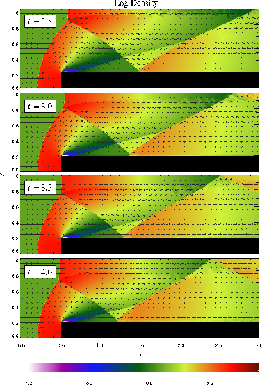
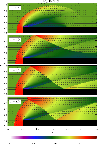
Until ![]() , the flow is unsteady, exhibiting multiple shock
reflections and interactions between different types of
discontinuities. Figure 35.19 shows the evolution of
density and velocity between
, the flow is unsteady, exhibiting multiple shock
reflections and interactions between different types of
discontinuities. Figure 35.19 shows the evolution of
density and velocity between ![]() and
and ![]() (the period considered
by Woodward and Colella). Immediately, a shock forms directly in
front of the step and begins to move slowly away from it.
Simultaneously, the shock curves around the corner of the step,
extending farther downstream and growing in size until it strikes
the upper boundary just after
(the period considered
by Woodward and Colella). Immediately, a shock forms directly in
front of the step and begins to move slowly away from it.
Simultaneously, the shock curves around the corner of the step,
extending farther downstream and growing in size until it strikes
the upper boundary just after ![]() . The corner of the step
becomes a singular point, with a rarefaction fan connecting the
still gas just above the step to the shocked gas in front of it.
Entropy errors generated in the vicinity of this singular point
produce a numerical boundary layer about one cell thick along the
surface of the step. Woodward and Colella reduce this effect by
resetting the cells immediately behind the corner to conserve
entropy and the sum of enthalpy and specific kinetic energy through
the rarefaction. However, we are less interested here in reproducing
the exact solution than in verifying the code and examining the
behavior of such numerical effects as resolution is increased, so we
do not apply this additional boundary condition. The errors near the
corner result in a slight over-expansion of the gas there and a weak
oblique shock where this gas flows back toward the step. At all
resolutions we also see interactions between the numerical boundary
layer and the reflected shocks that appear later in the calculation.
. The corner of the step
becomes a singular point, with a rarefaction fan connecting the
still gas just above the step to the shocked gas in front of it.
Entropy errors generated in the vicinity of this singular point
produce a numerical boundary layer about one cell thick along the
surface of the step. Woodward and Colella reduce this effect by
resetting the cells immediately behind the corner to conserve
entropy and the sum of enthalpy and specific kinetic energy through
the rarefaction. However, we are less interested here in reproducing
the exact solution than in verifying the code and examining the
behavior of such numerical effects as resolution is increased, so we
do not apply this additional boundary condition. The errors near the
corner result in a slight over-expansion of the gas there and a weak
oblique shock where this gas flows back toward the step. At all
resolutions we also see interactions between the numerical boundary
layer and the reflected shocks that appear later in the calculation.
The shock reaches the top wall at
![]() . The point of
reflection begins at
. The point of
reflection begins at
![]() and then moves to the left,
reaching
and then moves to the left,
reaching
![]() at
at ![]() . As it moves, the angle between
the incident shock and the wall increases until
. As it moves, the angle between
the incident shock and the wall increases until ![]() , at which
point it exceeds the maximum angle for regular reflection
(
, at which
point it exceeds the maximum angle for regular reflection
(![]() for
for
![]() ) and begins to form a Mach stem.
Meanwhile the reflected shock has itself reflected from the top of
the step, and here too the point of intersection moves leftward,
reaching
) and begins to form a Mach stem.
Meanwhile the reflected shock has itself reflected from the top of
the step, and here too the point of intersection moves leftward,
reaching
![]() by
by ![]() . The second reflection propagates
back toward the top of the grid, reaching it at
. The second reflection propagates
back toward the top of the grid, reaching it at ![]() and forming
a third reflection. By this time in low-resolution runs, we see a
second Mach stem forming at the shock reflection from the top of the
step; this results from the interaction of the shock with the
numerical boundary layer, which causes the angle of incidence to
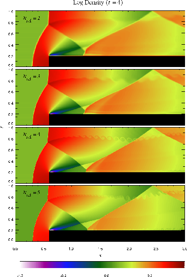
increase faster than in the converged solution. Figure 35.20 compares the density field at
and forming
a third reflection. By this time in low-resolution runs, we see a
second Mach stem forming at the shock reflection from the top of the
step; this results from the interaction of the shock with the
numerical boundary layer, which causes the angle of incidence to
increase faster than in the converged solution. Figure 35.20 compares the density field at ![]() as computed
by FLASH using several different maximum levels of refinement. Note
that the size of the artificial Mach reflection diminishes as
resolution improves.
as computed
by FLASH using several different maximum levels of refinement. Note
that the size of the artificial Mach reflection diminishes as
resolution improves.
|
|
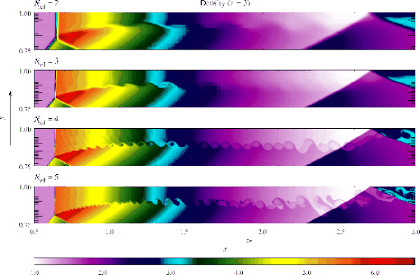
The shear cell behind the first (“real”) Mach stem produces
another interesting numerical effect, visible at ![]() --
Kelvin-Helmholtz amplification of numerical errors generated at the
shock intersection. The waves thus generated propagate downstream
and are refracted by the second and third reflected shocks. This
effect is also seen in the calculations of Woodward and Colella,
although their resolution was too low to capture the detailed eddy
structure we see. Figure 35.21 shows the detail of
this structure at
--
Kelvin-Helmholtz amplification of numerical errors generated at the
shock intersection. The waves thus generated propagate downstream
and are refracted by the second and third reflected shocks. This
effect is also seen in the calculations of Woodward and Colella,
although their resolution was too low to capture the detailed eddy
structure we see. Figure 35.21 shows the detail of
this structure at ![]() on grids with several different levels of
refinement. The effect does not disappear with increasing
resolution, for three reasons. First, the instability amplifies
numerical errors generated at the shock intersection, no matter how
small. Second, PPM captures the slowly moving, nearly vertical Mach
stem with only 1-2 cells on any grid, so as it moves from one
column of cells to the next, artificial kinks form near the
intersection, providing the seed perturbation for the instability.
Third, the effect of numerical viscosity, which can diffuse away
instabilities on course grids, is greatly reduced at high
resolution. This effect can be reduced by using a small amount of
extra dissipation to smear out the shock, as discussed by Colella
and Woodward (1984). This tendency of physical instabilities to
amplify numerical noise vividly demonstrates the need to exercise
caution when interpreting features in supposedly converged
calculations.
on grids with several different levels of
refinement. The effect does not disappear with increasing
resolution, for three reasons. First, the instability amplifies
numerical errors generated at the shock intersection, no matter how
small. Second, PPM captures the slowly moving, nearly vertical Mach
stem with only 1-2 cells on any grid, so as it moves from one
column of cells to the next, artificial kinks form near the
intersection, providing the seed perturbation for the instability.
Third, the effect of numerical viscosity, which can diffuse away
instabilities on course grids, is greatly reduced at high
resolution. This effect can be reduced by using a small amount of
extra dissipation to smear out the shock, as discussed by Colella
and Woodward (1984). This tendency of physical instabilities to
amplify numerical noise vividly demonstrates the need to exercise
caution when interpreting features in supposedly converged
calculations.
| Variable | Type | Default | Description |
| sim_pAmbient | real | 1 | Ambient pressure ( |
| sim_rhoAmbient | real | 1.4 | Ambient density ( |
| sim_windVel | real | 3 | Inflow velocity ( |
The Shu-Osher problem (Shu and Osher, 1989) tests a shock-capturing scheme's ability to resolve small-scale flow features. It gives a good indication of the numerical (artificial) viscosity of a method. Since it is designed to test shock-capturing schemes, the equations of interest are the one-dimensional Euler equations for a single-species perfect gas.
In this problem, a (nominally) Mach 3 shock wave propagates into a sinusoidal density field. As the shock advances, two sets of density features appear behind the shock. One set has the same spatial frequency as the unshocked perturbations, but for the second set, the frequency is doubled. Furthermore, the second set follows more closely behind the shock. None of these features is spurious. The test of the numerical method is to accurately resolve the dynamics and strengths of the oscillations behind the shock.
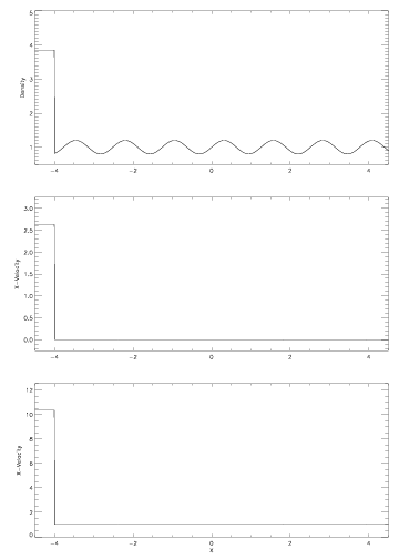
The shu_osher problem is initialized as follows.
On the domain
![]() , the shock is at
, the shock is at
![]() at
at
![]() .
On either side of the shock,
.
On either side of the shock,
 |
(35.14) |
The problem is strictly one-dimensional; building 2-d or 3-d executables
should give the same results along each ![]() -direction grid line. For
this problem, special boundary conditions are applied. The initial
conditions should not change at the boundaries; if they do, errors
at the boundaries can contaminate the results. To avoid this
possibility, a boundary condition subroutine was written to set the
boundary values to their initial values.
-direction grid line. For
this problem, special boundary conditions are applied. The initial
conditions should not change at the boundaries; if they do, errors
at the boundaries can contaminate the results. To avoid this
possibility, a boundary condition subroutine was written to set the
boundary values to their initial values.
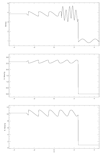
The purpose of the tests is to determine how much resolution, in
terms of mesh cells per feature, a particular method requires to
accurately represent small scale flow features. Therefore, all
computations are carried out on equispaced meshes without
adaptive refinement. Solutions are obtained at ![]() . The
reference solution, using 3200 mesh cells, is shown in
Figure 35.23. This solution was
computed using PPM at a CFL number of 0.8. Note the shock located at
. The
reference solution, using 3200 mesh cells, is shown in
Figure 35.23. This solution was
computed using PPM at a CFL number of 0.8. Note the shock located at
![]() , and the high frequency density oscillations just to
the left of the shock. When the grid resolution is insufficient,
shock-capturing schemes underpredict the amplitude of these
oscillations and may distort their shape.
, and the high frequency density oscillations just to
the left of the shock. When the grid resolution is insufficient,
shock-capturing schemes underpredict the amplitude of these
oscillations and may distort their shape.
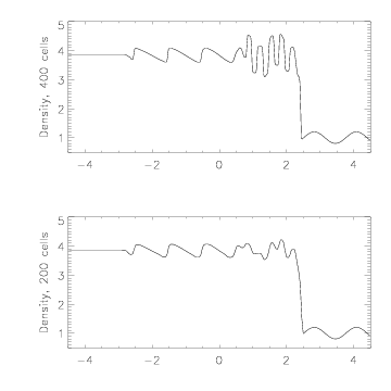
Figure 35.24 shows the density field for the same scheme at 400 mesh cells and at 200 mesh cells. With 400 cells, the amplitudes are only slightly reduced compared to the reference solution; however, the shapes of the oscillations have been distorted. The slopes are steeper and the peaks and troughs are broader, which is the result of overcompression from the contact-steepening part of the PPM algorithm. For the solution on 200 mesh cells, the amplitudes of the high-frequency oscillations are significantly underpredicted.
| Variable | Type | Value | Description |
| st_stirmax | real | 25.1327 | maximum stirring wavenumber |
| st_stirmin | real | 6.2832 | minimum stirring wavenumber |
| st_energy | real | 5.E-6 | energy input per mode |
| st_decay | real | 0.5 | correlation time for driving |
| st_freq | integer | 1 | frequency of stirring |
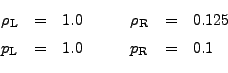
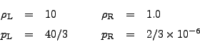
We construct the initial conditions for the relativistic shock tube problem as
found in Martí & Müller (2003). We use an ideal equation of state
with
![]() for this problem and the left and right states are given:
for this problem and the left and right states are given:
 |
(35.15) |
and the computational domain is
![]() . The initial
shock location is at
. The initial
shock location is at ![]() (halfway across a box with unit dimensions).
(halfway across a box with unit dimensions).
In FLASH, the RHD Sod problem (RHD_Sod) uses the runtime parameters listed in Table 35.9:
| Variable | Type | Default | Description |
| sim_rhoLeft | real | 10 | Initial density to the
left of the interface
(
|
| sim_rhoRight | real | 1.0 | Initial density to the
right (
|
| sim_pLeft | real | 40/3 | Initial pressure to the
left ( |
| sim_pRight | real |
|
Initial pressure to the
right ( |
| sim_uLeft | real | 0 | Initial velocity
(perpendicular to interface)
to the left ( |
| sim_uRight | real | 0 | Initial velocity
(perpendicular to interface)
to the right ( |
| sim_xangle | real | 0 | Angle made by interface
normal with the |
| sim_yangle | real | 90 | Angle made by interface
normal with the |
| sim_posn | real | 0.5 | Point of intersection between
the interface plane and the
|
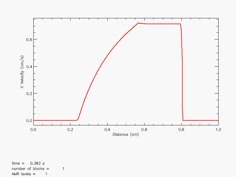
Figure 35.27, Figure 35.28, and Figure 35.29 show the results of running
the RHD Sod problem on a one-dimensional uniform grid of size 400 at simulation time ![]() In this run the
left-going wave is the rarefaction wave, while two right-going waves are the contact discontinuity and the
shock wave. This configuration results in mildly relativistic effects that are mainly thermodynamical in nature.
In this run the
left-going wave is the rarefaction wave, while two right-going waves are the contact discontinuity and the
shock wave. This configuration results in mildly relativistic effects that are mainly thermodynamical in nature.
The differences in the relativistic regime, as compared to Newtonian hydrodynamics, can be seen in a curved velocity profile for the rarefaction wave and the narrow constant state (density shell) in between the shock wave and contact discontinuity. Numerically, it is particularly challenging to resolve the thin narrow density plateau, which is bounded by a leading shock front and a trailing contact discontinuity (see Figure 35.27).
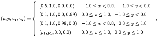 |
(35.16) |
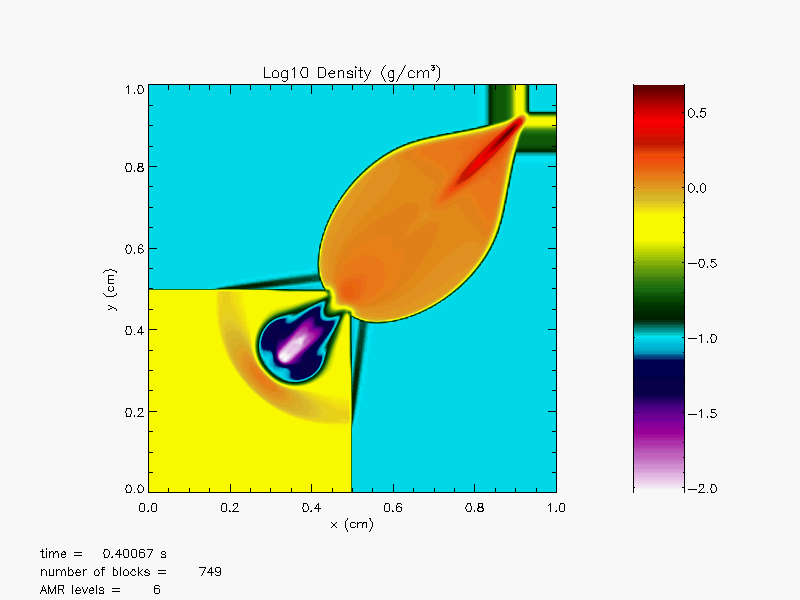
The solution obtained at ![]() in Figure 35.30 shows that
the symmetry of the problem is well maintained. The two shocks are propagated
from the upper left and the lower right regions to the upper right region, yielding
continuous collisions of shocks at the upper right corner.The curved shock fronts are
transmitted and formed in the diagonal region of the domain. The lower left region is
bounded by contact discontinuities. By the time
in Figure 35.30 shows that
the symmetry of the problem is well maintained. The two shocks are propagated
from the upper left and the lower right regions to the upper right region, yielding
continuous collisions of shocks at the upper right corner.The curved shock fronts are
transmitted and formed in the diagonal region of the domain. The lower left region is
bounded by contact discontinuities. By the time ![]() most of regions are filled with
shocked gas, whereas there are still two unperturbed regions in the lower left and
upper right regions.
most of regions are filled with
shocked gas, whereas there are still two unperturbed regions in the lower left and
upper right regions.
|
Plots in Figure 35.31(a) - Figure 35.33(b) illusrate
Mach number and pressure plots over the airfoil with the three different initial Mach numbers, 0.65, 0.95 and 1.2 at ![]() By this time, the flow conditions have reached their steady states. For Mach number = 0.65, the critical Mach number has not yet
been obtained and the flow over the airfoil is all subsonic as shown in Figure 35.31(a). Since the airfoil is
asymmetric and cambered, we see there are pressure gradients across the top and bottom surfaces
even at zero angle of attack in Figure 35.31(b).
These pressure gradients (higher pressure at the bottom than the top) generate a lift force
by which an airplane can fly defying gravity.
By this time, the flow conditions have reached their steady states. For Mach number = 0.65, the critical Mach number has not yet
been obtained and the flow over the airfoil is all subsonic as shown in Figure 35.31(a). Since the airfoil is
asymmetric and cambered, we see there are pressure gradients across the top and bottom surfaces
even at zero angle of attack in Figure 35.31(b).
These pressure gradients (higher pressure at the bottom than the top) generate a lift force
by which an airplane can fly defying gravity.
At Mach number reaching 0.95 as shown in Figure 35.32(a) there are local points that are supersonic. This indicates that the critical Mach number for the airfoil is between 0.65 and 0.95. In fact, one can show that the critical Mach number is around 0.7 for the NACA2412 airfoil. We see that there is a development of a bow shock formation in front of the airfoil. A formation of a subsonic region between the bow shock and the nose of the airfoil is visible in the Mach number plot. Inside the bow shock, a sonic line at which the local flow speed becomes the sound speed makes an oval shape together with the bow shock. In both the Mach number and pressure plots, a strong wake forms starting from the top and bottom of the surfaces near the trailing edge. The wake is hardly visible for Mach number 0.65 in Figure 35.31(a) and Figure 35.31(b). Normal shock waves have formed steming from the trailing edge as seen in Figure 35.32(a) and Figure 35.32(b).
At Mach number 1.2 the flow becomes supersonic everywhere. In this case, the shape of the bow shock becomes narrower and there are much larger supersonic pockets developed on the top and bottom surfaces with a smaller subsonic region between the bow shock and the nose region.
|
[a] 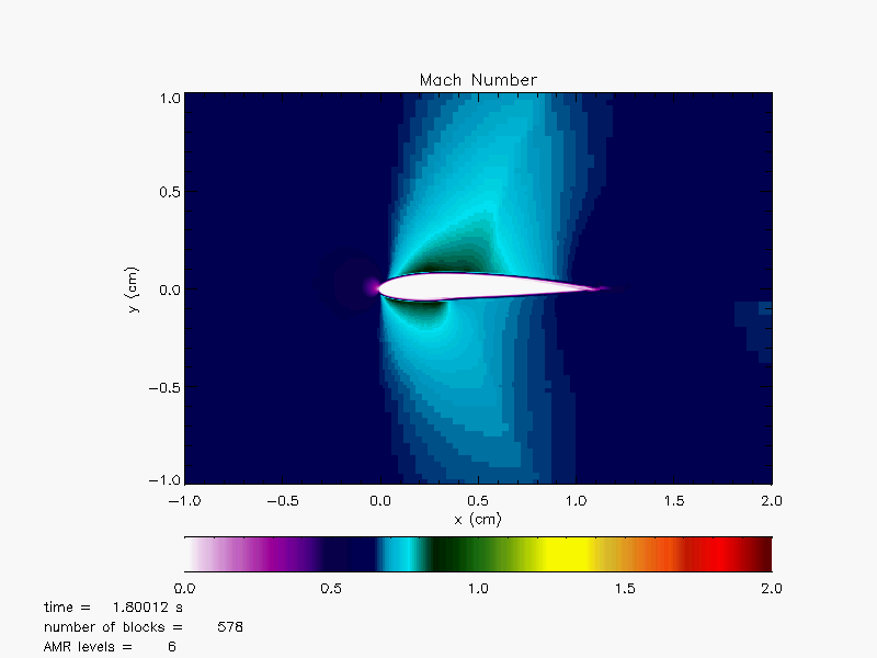 [b]
[b] 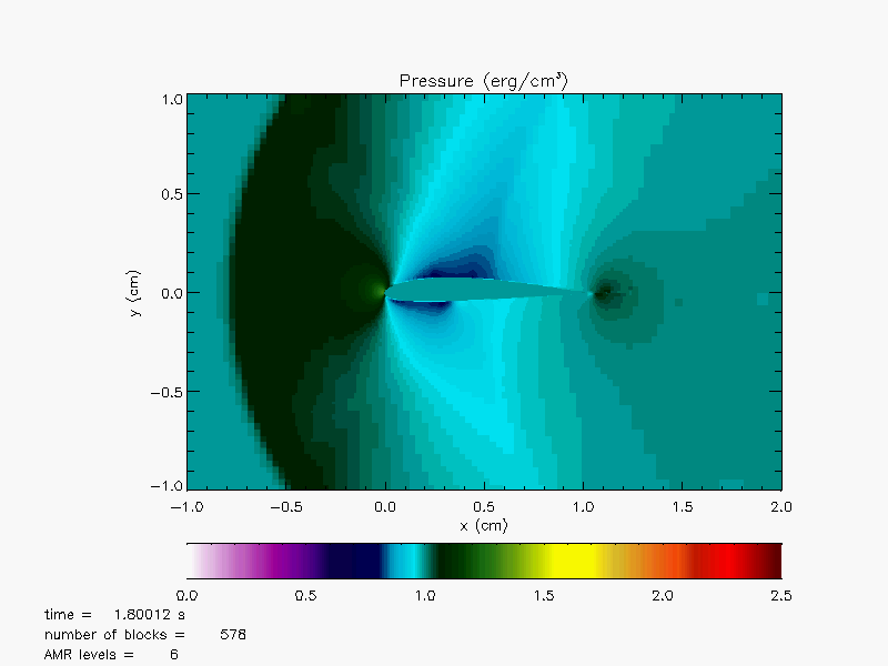
|
|
[a] 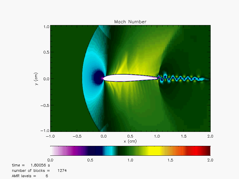 [b]
[b] 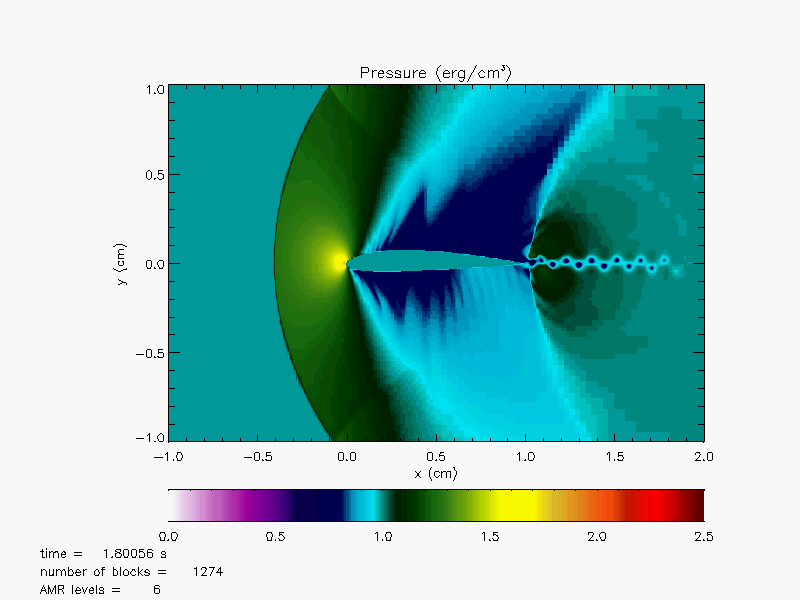
|
|
[a] 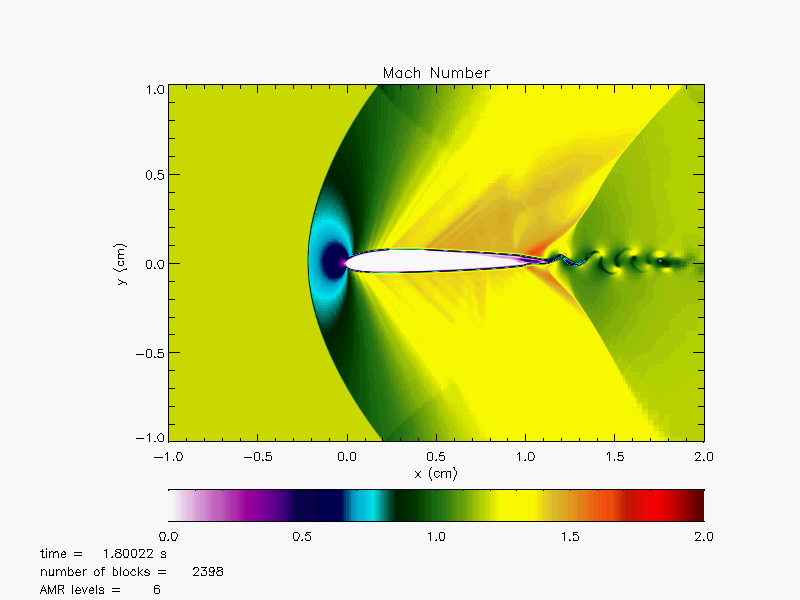 [b]
[b] 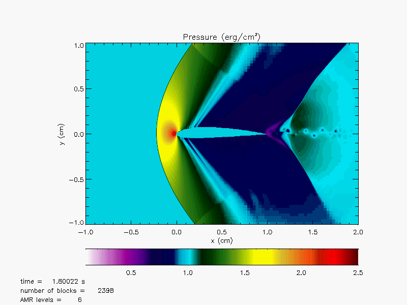
|
One important thing in this problem is to keep the given symmetry throughout the simulation. The flow symmetry across the diagonal direction is well preseved in Figure 35.34(a) and Figure 35.34(b).
|
[a] 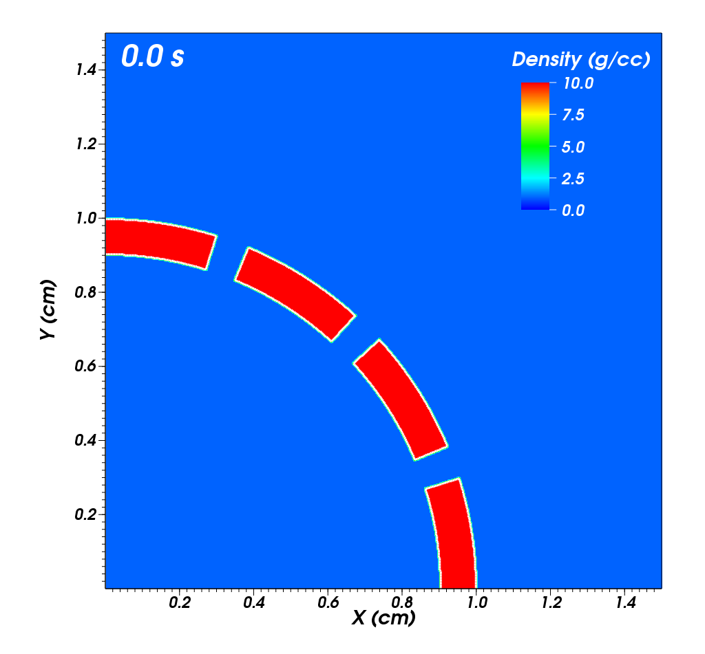 [b]
[b] 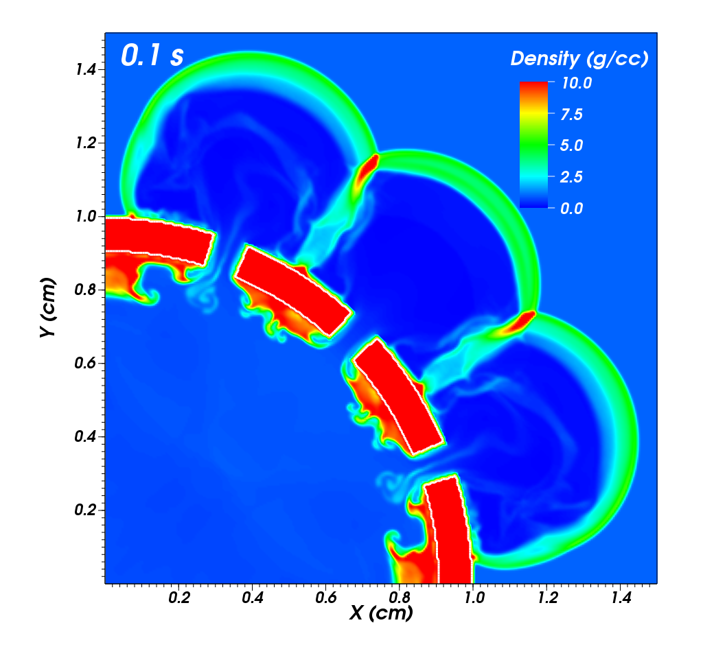
|