Next: 35.1 Hydrodynamics Test Problems Up: IX. Simulation Units Previous: IX. Simulation Units Contents Index
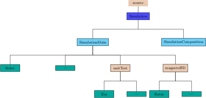 |
To verify that FLASH works as expected and to debug changes in the code, we have created a suite of standard test problems. Many of these problems have analytical solutions that can be used to test the accuracy of the code. Most of the problems that do not have analytical solutions produce well-defined flow features that have been verified by experiments and are stringent tests of the code. For the remaining problems, converged solutions, which can be used to test the accuracy of lower resolution simulations, are easy to obtain. The test suite configuration code is included with the FLASH source tree (in the Simulation/ directory), so it is easy to configure and run FLASH with any of these problems `out of the box.' Sample runtime parameter files are also included. All the test problems reside in the Simulations unit. The unit provides some general interfaces most of which do not have general implementations. Each application provides its own implementation for these interfaces, for example, Simulation_initBlock. The exception is Simulation_initSpecies, which provides general implementations for different classes of problems.