8.9 GridParticles

Figure 8.8: The Grid unit: structure of GridParticles subunit.

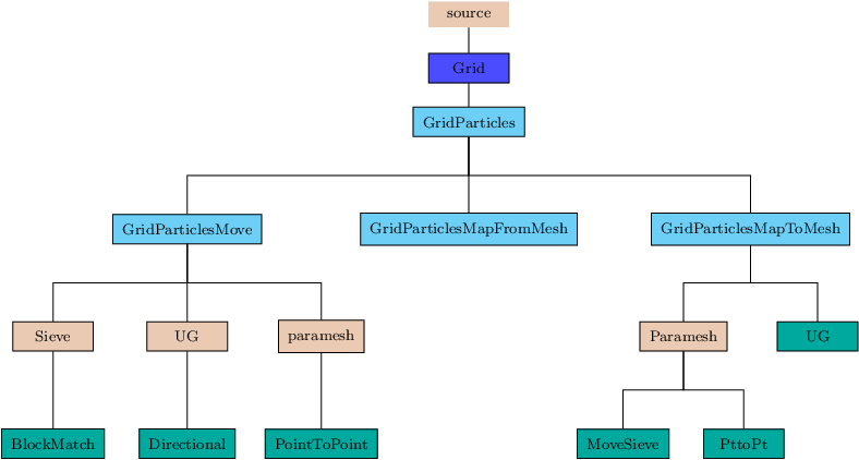
FLASH is primarily an Eulerian code, however, there is support for tracing the flow using Lagrangian particles. In FLASH4 we have generalized the interfaces in the Lagrangian framework of the Grid unit in such a way that it can also be used for miscellaneous non-Eulerian data such as tracing the path of a ray through the domain, or tracking the motion of solid bodies immersed in the fluid. FLASH also uses active particles with mass in cosmological simulations, and charged particles in a hybrid PIC solver. Each particle has an associated data structure, which contains fields such as its physical position and velocity, and relevant physical attributes such as mass or field values in active particles. Depending upon the time advance method, there may be other fields to store intermediate values. Also, depending upon the requirements of the simulation, other physical variables such as temperature etc.  may be added to the data structure. The GridParticles subunit of the Grid unit has two sub-subunits of its own. The GridParticlesMove sub-subunit moves the data structures associated with individual particles when the particles move between blocks; the actual movement of the particles through time advancement is the responsibility of the Particles unit. Particles move from one block to another when their time advance places them outside their current block. In AMR, the particles can also change their block through the process of refinement and derefinement. The GridParticlesMap sub-subunit provides mapping between particles data and the mesh variables. The mesh variables are either cell-centered or face-centered, whereas a particle's position could be anywhere in the cell. The GridParticlesMap sub-subunit calculates the particle's properties at its position from the corresponding mesh variable values in the appropriate cell . When using active particles, this sub-subunit also maps the mass of the particles onto the specified mesh variable in appropriate cells. The next sections describe the algorithms for moving and mapping particles data.

8.9.1 GridParticlesMove

FLASH4 has implementations of three different parallel algorithms for moving the particles data when they are displaced from their current block. FLASH3 had an additional algorithm, Perfect Tree Level which made use of the oct-tree structure. However, because in all performance experiments it performed significantly worse than the other two algorithms, it is not supported currently in FLASH4. The simplest algorithm, Directional algorithm is applicable only to the uniform grid when it is configured with one block per processor. This algorithm uses directional movement of data, and is easy because the directional neighbors are trivially known. The movement of particles data is much more challenging with AMR even when the grid is not refining. Since the blocks are at various levels of refinement at any given moment, a block may have more than one neighbor along one or more of its faces. The distribution of blocks based on space-filling curve is an added complication since the neighboring blocks along a face may reside at a non-neighboring processor The remaining two algorithmss included in FLASH4 implement GridParticlesMove subunit for the adaptive mesh; Point to Point and Sieve, of which only the Sieve algorithm is able to move the data when the mesh refines. Thus even when a user opts for the PointToPoint implementation for moving particles with time evolution, some part of the Sieve implementation must necessarily be included to successfully move the data upon refinement.

8.9.1.1 Directional Move

The Directional Move algorithm for moving particles in a Uniform Grid minimizes the number of communication steps instead of minimizing the volume of data moved. Its implementation has the following steps:

1. Scan particle positions. Place all particles with their $x$ coordinate value greater than the block bounding box in the Rightmove bin, and place those with $x$ coordinate less than block bounding box in Leftmove bin.
2. Exchange contents of Rightbin with the right block neighbor's Leftbin contents, and those of the Leftbin with left neightbor's Rightbin contents.
3. Merge newly arrived particles from step 2 with those which did not move outside their original block.
4. Repeat steps 1-3 for the y direction.
5. Repeat step 1-2 for the z direaction.

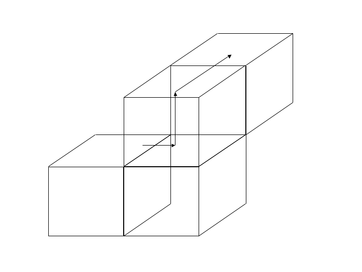
At the end of these steps, all particles will have reached their destination blocks, including those that move to a neighbor on the corner. Figure 8.9 illustrates the steps in getting a particle to its correct destination.

Figure 8.9: Moving one particle to a neighbor on the corner.

8.9.1.2 Point To Point Algorithm

As a part of the data cached by Paramesh, there is wealth of information about the neighborhood of all the blocks on a processor. This information includes the processor and block number of all neighbors (face and corners) if they are at the same refinement level. If those neighbors are at lower refinement level, then the neighbor block is in reality the current block's parent's neighbor, and the parent's neighborhood information is part of the cached data. Similarly, if the neighbor is at a higher resolution then the current blocks neighbor is in reality the parent of the neighbor. The parent's metadata is also cached, from which information about all of its children can be derived. Thus it is possible to determine the processor and block number of the destination block for each particle. The PointToPoint implementation finds out the destinations for every particles that is getting displaced from its block. Particles going to local destination blocks are moved first. The remaining particles are sorted based on their destination processor number, followed by a couple of global operations that allow every processor to determine the number of particles it is expected to receive from all of the other processors. A processor then posts asynchronous receives for every source processor that had at least one particle to send to it. In the next step, the processor cycles through the sorted list of particles and sends them to the appropriate destinations using synchronous mode of communition.

8.9.1.3 Sieve Algorithm

The Sieve algorithm does not concern itself with the configuration of the underlying mesh at any time. It also does not distinguish between data movements due to time evolution or regridding, and is therefore the only usable implementation when the particles are displaced as a consequence of mesh refinement. The sieve implementation works with two bins, one collects particles that have to be moved off-processor, and the other receives particles sent to it by other processors. The following steps broadly describe the algorithm:

1. For each particle, find if its current position is on the current block
2. If not, find if its current position is on another block on the same processor. If it is move the particle to that block, otherwise put it in the send bin.
3. Send contents of the send bin to the designated neighbor, and receive contents of another neighbor's send bin into my receive bin.
4. Repeat step 2 on the contents of the receive bin, and step 3 until all particles are at their destination.
5. For every instance of step 3, the designated send and receive neighbors are different from any of the previous steps.

In this implementation, the trick is to use an algorithm to determine neighbors in such a way that all the particles reach their destination in minimal number of hops. Using $MyPE+n*(-1)^{n+1}$ as the destination processor and $MyPE+n*(-1)^{n}$ as the source processor in modulo $numProcs$ arithmetic meets the requirements. Here $MyPE$ is the local processor number and $numProcs$ is the number of processors.

8.9.2 GridParticlesMapToMesh

FLASH4 provides support for particles that can experience forces and contribute to the problem dynamics. These are termed active particles, and are described in detail in Chp:Particles. As these particles may move independently of fluid flow, it is necessary to update the grid by mapping an attribute of the particles to the cells of the grid. We use these routines, for example, during the PM method to assign the particles' mass to the particle density solution variable pden. The hybrid PIC method uses its own variation for mapping appropriate physical quantities to the mesh.

In general the mapping is performed using the grid routines in the GridParticlesMapToMesh directory and the particle routines in the ParticlesMapping directory. Here, the particle subroutines map the particles' attribute into a temporary array which is independent of the current state of the grid, and the grid subroutines accumulate the mapping from the array into valid cells of the computational domain. This means the grid subroutines accumulate the data according to the grid block layout, the block refinement details, and the simulation boundary conditions. As these details are closely tied with the underlying grid, there are separate implementations of the grid mapping routines for UG and PARAMESH simulations.

The implementations are required to communicate information in a relatively non-standard way. Generally, domain decomposition parallel programs do not write to the guard cells of a block, and only use the guard cells to represent a sufficient section of the domain for the current calculation. To repeat the calculation for the next time step, the values in the guard cells are refreshed by taking updated values from the internal section of the relevant block. In FLASH4, PARAMESH refreshes the values in the guard cells automatically, and when instructed by a Grid_fillGuardCells call.

In contrast, the guard cell values are mutable in the particle mapping problem. Here, it is possible that a portion of the particle's attribute is accumulated in a guard cell which represents an internal cell of another block. This means the value in the updated guard cell must be communicated to the appropriate block. Unfortunately, the mechanism to communicate information in this direction is not provided by PARAMESH or UG grid. As such, the relevant communication is performed within the grid mapping subroutines directly.

In both PARAMESH and UG implementations, the particles' attribute is “smeared” across a temporary array by the generic particle mapping subroutine. Here, the temporary array represents a single leaf block from the local processor. In simulations using the PARAMESH grid, the temporary array represents each LEAF block from the local processor in turn. We assign a particle's attribute to the temporary array when that particle exists in the same space as the current leaf block. For details about the attribute assignment schemes available to the particle mapping sub-unit, please refer to Sec:Particles Mapping.

After particle assignment, the Grid sub-unit applies simulation boundary conditions to those temporary arrays that represent blocks next to external boundaries. This may change the quantity and location of particle assignment in the elements of the temporary array. The final step in the process involves accumulating values from the temporary array into the correct cells of the computational domain. As mentioned previously, there are different strategies for UG and PARAMESH grids, which are described in Sec:UniformGridParticleMap and Sec:ParameshGridParticleMap, respectively.

FLASH3 Transition: The particle mapping routines can be run in a custom debug mode which can help spot data errors (and even detect possible bugs). In this mode we inspect data for inconsistencies. To use, append the following line to the setup script:  

-defines=DEBUG_GRIDMAPPARTICLES

8.9.2.1 Uniform Grid

The Uniform Grid algorithm for accumulating particles' attribute on the grid is similar to the particle redistribution algorithm described in Sec: ug_algorithm. We once again apply the concept of directional movement to minimize the number of communication steps:

1. Take the accumulated temporary array and iterate over all elements that correspond to the x-axis guard cells of the low block face. If a guard cell has been updated, determine its position in the neighboring block of the low block face. Copy the guard cell value and a value which encodes the destination cell into the send buffer.
2. Send the buffer to the low-side processor, and receive a buffer from the high-side processor. For processors next to a domain boundary assume periodic conditions because all processors must participate. If the simulation does not have periodic boundary conditions, there is still periodic communication at the boundaries, but the send buffers do not contain data.
3. Iterate over the elements in the receive buffer and accumulate the values into the local temporary array at the designated cells. It is possible to accumulate values in cells that represent internal cells and guard cells. A value accumulated in a guard cell will be repacked into the send buffer during the next directional (y or z) sweep.
4. Repeat steps 1-3 for the high block face.
5. Repeat steps 1-4 for the y-axis, and then the z-axis.

When the guard cell's value is packed into the send buffer, a single value is also packed which is a 1-dimensional representation of the destination cell's N-dimensional position. The value is obtained by using an array equation similar to that used by a compiler when mapping an array into contiguous memory. The receiving processor applies a reverse array equation to translate the value into N-dimensional space. The use of this communication protocol is designed to minimize the message size.

At the end of communication, each local temporary buffer contains accumulated values from guard cells of another block. The temporary buffer is then copied into the solution array.

8.9.2.2 Paramesh Grid

There are two implementations of the AMR algorithms for accumulating particles' attribute on the grid. They are inspired by a particle redistribution algorithms Sieve and Point to Point described in Sec: sieve_algorithm and Sec: ptop_algorithm respectively.

The MoveSieve implementation of the mapping algorithm uses the same back and forth communication pattern as Sieve to minimize the number of message exchanges. That is, processor $MyPE$ sends to $MyPE+n*(-1)^{n+1}$ and receives from $MyPE+n*(-1)^{n}$, where, $MyPE$ is the local processor number and $n$ is the count of the buffer exchange round. As such, this communication pattern involves a processor exchanging data with its nearest neighbor processors first. This is appropriate here because the block distribution generated by the space filling curve should be high in data locality, i.e., nearest neighbor blocks should be placed on the same processor or nearest neighbor processors.

Similarly, the Point to Point implementation of the mapping algorithm exploits the cached neighborhood knowledge, and uses a judicious combination of global communications with asynchronous receives and synchronous sends, as described in Sec: ptop_algorithm. Other than their communication patterns, the two implementations are very similar as described below.

1. Accumulate the temporary array values into the central section of the corresponding leaf block.
2. Divide the leaf block guard cells into guard cell regions. Determine whether the neighbor(s) to a particular guard cell region exist on the same processor.
3. If a neighbor exists on the same processor, the temporary array values are accumulated into the central cells of that leaf block. If the neighbor exists off processor, all temporary array values corresponding to a single guard cell region are copied into a send buffer. Metadata is also packed into the send buffer which describes the destination of the updated values.
4. Repeat steps 1-3 for each leaf block.
5. Carry out data exchange with off-processor destinations as described in the Sec: sieve_algorithm or Sec: ptop_algorithm

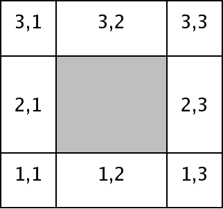
The guard cell region decomposition described in Step 2 is illustrated in Figure 8.10. Here, the clear regions correspond to guard cells and the gray region corresponds to internal cells. Each guard cell region contains cells which correspond to the internal cells of a single neighboring block at the same refinement.

Figure 8.10: A single 2-D block showing how guard cells are divided into regions.

We use this decomposition as it makes it possible to query public PARAMESH data structures which contain the block and process identifier of the neighboring block at the same refinement. However, at times this is not enough information for finding the block neighbor(s) in a refined grid. We therefore categorize neighboring blocks as: Existing on the same processor, existing on another processor and the block and process ID are known, and existing on another processor and the block and process ID are unknown. If the block and process identifier are unknown we use the FLASH4 corner ID. This is a viable alternative as the corner ID of a neighboring block can always be determined.

The search process also identifies the refinement level of the neighboring block(s). This is important as the guard cell values cannot be directly accumulated into the internal cells of another block if the blocks are at a different refinement levels. Instead the values must be operated on in processes known as restriction and prolongation (see Sec:gridinterp). We perform these operations directly in the GridParticlesMapToMesh routines, and use quadratic interpolation during prolongation.

Guard cell data is accumulated in blocks existing on the same processor, or packed into a send buffer ready for communication. When packed into the send buffer, we keep values belonging to the same guard cell region together. This enables us to describe a whole region of guard cell data by a small amount of metadata. The metadata consists of: Destination block ID, destination processor ID, block refinement level difference, destination block corner ID (IAXIS, JAXIS, KAXIS) and start and end coordinates of destination cells (IAXIS, JAXIS, KAXIS). This is a valid technique because there are no gaps in the guard cell region, and is sufficient information for a receiving processor to unpack the guard cell data correctly.

We size the send / receive buffers according to the amount of data that needs to be communicated between processors. This is dependent upon how the PARAMESH library distributes blocks to processors. Therefore, in order to size the communication buffers economically, we calculate the number of guard cells that will accumulate on blocks belonging to another processor. This involves iterating over every single guard cell region, and keeping a running total of the number of off-processor guard cells. This total is added to the metadata total to give the size of the send buffer required on each processor. We use the maximum of the send buffer size across all processors as the local size for the send / receive buffer. Choosing the maximum possible size prevents possible buffer overflow when an intermediate processor passes data onto another processor.

After the point to point communication in step 6, the receiving processor scans the destination processor identifier contained in each metadata block. If the data belongs to this processor it is unpacked and accumulated into the central cells of the relevant leaf block. As mentioned earlier, it is possible that some guard cell sections do not have the block and processor identifier. When this happens, the receiving processor attempts to find the same corner ID in one of its blocks by performing a linear search over each of its leaf blocks. Should there be a match, the guard cells are copied into the matched block. If there is no match, the guard cells are copied from the receive buffer into the send buffer, along with any guard cell region explicitly designated for another processor. The packing and unpacking will continue until all send buffers are empty, as indicated by the result of the collective communication.

It may seem that the algorithm is unnecessarily complicated, however, it is the only viable algorithm when the block and process identifiers of the nearest block neighbors are unknown. This is the situation in FLASH3.0, in which some data describing block and process identifiers are yet to be extracted from PARAMESH. As an aside, this is different to the strategy used in FLASH2, in which the entire PARAMESH tree structure was copied onto each processor. Keeping a local copy of the entire PARAMESH tree structure on each processor is an unscalable approach because increase in the levels of resolution increases the meta-data memory overhead, which restricts the size of active particle simulations. Therefore, Point to Point method is a better option for larger simulations, and significantly, simulations that run on massively parallel processing (MPP) hardware architectures.

In FLASH3.1 we added a routine which searches non-public PARAMESH data to obtain all neighboring block and process identifiers. This discovery greatly improves the particle mapping performance because we no longer need to perform local searches on each processor for blocks matching a particular corner ID.

As another consequence of this discovery, we are able to experiment with alternative mapping algorithms that require all block and process IDs. From FLASH3.1 on we also provide a non-blocking point to point implementation in which off-processor cells are sent directly to the appropriate processor. Here, processors receive messages at incremented positions along a data buffer. These messages can be received in any order, and their position in the data buffer can change from run to run. This is very significant because the mass accumulation on a particular cell can occur in any order, and therefore can result in machine precision discrepancies. Please be aware that this can actually lead to slight variations in end-results between two runs of the exact same simulation.