21. Particles Unit

Figure 21.1: The Particles unit main subunit.

Figure 21.2: The Particles unit with ParticlesInitialization and ParticlesMapping subunits.

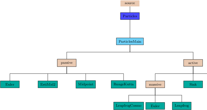
The support for particles in FLASH4 comes in two flavors, active and passive. Active particles are further classified into two categories; massive and charged. The active particles contribute to the dynamics of the simulation, while passive particles follow the motion of Lagrangian tracers and make no contribution to the dynamics. Particles are dimensionless objects characterized by positions ${\bf x}_i$, velocities ${\bf v}_i$, and sometimes other quantities such as mass $m_i$ or charge $q_i$ . Their characteristic quantities are considered to be defined at their positions and may be set by interpolation from the mesh or may be used to define mesh quantities by extrapolation. They move relative to the mesh and can travel from block to block, requiring communication patterns different from those used to transfer boundary information between processors for mesh-based data.

Passive particles acquire their kinematic information (velocities) directly from the mesh. They are meant to be used as passive flow tracers and do not make sense outside of a hydrodynamical context. The governing equation for the $i$th passive particle is particularly simple and requires only the time integration of interpolated mesh velocities.

$${d{\bf x}_i\over dt} = {\bf v}_i$$ (21.1)

Active particles experience forces and may themselves contribute to the problem dynamics (e.g., through long-range forces or through collisions). They may additionally have their own motion independent of the grid, so an additional motion equation of

$${\bf v}_i^{n+1} = {\bf v}_i^n + {\bf a}_i^n\Delta t^n .$$ (21.2)

may come into play. Here ${\bf a}_i$ is the particle acceleration. Solving for the motion of active particles is also referred to as solving the $N$-body problem. The equations of motion for the $i$th active particle include the equation (21.1) and another describing the effects of forces.

$$m_i{d{\bf v}_i\over dt} = {\bf F}_{{\rm lr,}i} + {\bf F}_{{\rm sr,}i} ,$$ (21.3)

Here, ${\bf F}_{{\rm lr,}i}$ represents the sum of all long-range forces (coupling all particles, except possibly those handled by the short-range term) acting on the $i$th particle and ${\bf F}_{{\rm sr,}i}$ represents the sum of all short-range forces (coupling only neighboring particles) acting on the particle.

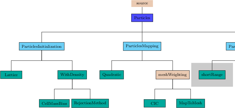
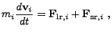
For both types of particles, the primary challenge is to integrate (21.1) forward through time. Many alternative integration methods are described in Section Sec:Particles Integration below. Additional information about the mesh to particle mapping is described in Sec:Particles Mapping. An introduction to the particle techniques used in FLASH is given by R. W. Hockney and J. W. Eastwood in Computer Simulation using Particles (Taylor and Francis, 1988).

FLASH3 Transition: Please note that the particles routines have not been thoroughly tested with non-Cartesian coordinates; use them at your own risk!

New since FLASH3.1: Since release 3.1 of FLASH, a single simulation can have both active and passive particles defined. FLASH3 and FLASH2 allowed only active or passive particles in a simulation. Because of the added complexity, new Config syntax and new setup script syntax is necessary for Particles. See Sec:ListSetupArgs for command line options, Sec:FlashHparticles for Config sytax, and Sec:ParticlesUsing below for more details.

FLASH4 includes support for sink particles. These are a special kind of (massive) active particles, with special rules for creation, mass accretion, and interaction with fluid variables and other particles. See Sec:Particles Sink below for information specific to sink particles.