21.1 Time Integration

The active and passive particles have many different time integration schemes available. The subroutine Particles_advance handles the movement of particles through space and time. Because FLASH4 has support for including different types of both active and passive particles in a single simulation, the implementation of Particles_advance may call several helper routines of the form pt_advanceMETHOD (e.g., pt_advanceLeapfrog, pt_advanceEuler_active, pt_advanceCustom), each acting on an appropriate subset of existing particles. The METHOD here is determined by the ADVMETHOD part of the PARTICLETYPE Config statement (or the ADV par of a -particlemethods setup option) for the type of particle. See the Particles_advance source code for the mapping from ADVMETHOD keyword to pt_advanceMETHOD subroutine call.

21.1.1 Active Particles (Massive)

The active particles implementation includes different time integration schemes, long-range force laws (coupling all particles), and short-range force laws (coupling nearby particles). The attributes listed in Table 21.1 are provided by this subunit. A specific implementation of the active portion of Particles_advance is selected by a setup option such as -with-unit=Particles/ParticlesMain/active/massive/Leapfrog, or by specifying something like REQUIRES Particles/ParticlesMain/active/massive/Leapfrog in a simulation's Config file (or by listing the path in the Units file if not using the -auto configuration option). Further details are given is Sec:ParticlesUsing below.

Available time integration schemes for active particles include

• Forward Euler. Particles are advanced in time from $t^n$ to $t^{n+1} = t^n + \Delta t^n$ using the following difference equations:
  

  $${\bf x}_i^{n+1} = {\bf x}_i^n + {\bf v}_i^n\Delta t^n$$

  $${\bf v}_i^{n+1} = {\bf v}_i^n + {\bf a}_i^n\Delta t^n .$$ (21.4)

  
  Here ${\bf a}_i$ is the particle acceleration. Within FLASH4, this scheme is implemented in Particles/ParticlesMain/active/massive/Euler. This Euler scheme (as well as the Euler scheme for the passive particles) is first-order accurate and is included for testing purposes only. It should not be used in a production run.

• Variable-timestep leapfrog. Particles are advanced using the following difference equations
  

  $${\bf x}_i^1 = {\bf x}_i^0 + {\bf v}_i^0\Delta t^0$$

  $${\bf v}_i^{1/2} = {\bf v}_i^0 + {1\over2}{\bf a}_i^0\Delta t^0$$ (21.5)

  $${\bf v}_i^{n+1/2} = {\bf v}_i^{n-1/2} + C_n{\bf a}_i^n + D_n{\bf a}_i^{n-1}$$

  $${\bf x}_i^{n+1} = {\bf x}_i^n + {\bf v}_i^{n+1/2}\Delta t^n .$$

  
  The coefficients $C_n$ and $D_n$ are given by
  

  $$C_n = {1\over2}\Delta t^n + {1\over3}\Delta t^{n-1} + {1\over6}\left({{\Delta t^n}^2\over\Delta t^{n-1}}\right)$$

  $$D_n = {1\over6}\left(\Delta t^{n-1} - {{\Delta t^n}^2\over\Delta t^{n-1}}\right) .$$ (21.6)

  
  By using time-centered velocities and stored accelerations, this method achieves second-order time accuracy even with variable timesteps. Within FLASH4, this scheme is implemented in Particles/ParticlesMain/active/massive/Leapfrog

• Cosmological variable-timestep leapfrog. (Particles/ParticlesMain/active/massive/LeapfrogCosmo) The coefficients in the leapfrog update are modified to take into account the effect of cosmological redshift on the particles. The particle positions ${\bf x}$ are interpreted as comoving positions, and the particle velocities ${\bf v}$ are interpreted as comoving peculiar velocities ( ${\bf v} = {\dot{\bf x}}$). The resulting update steps are
  

  $${\bf x}_i^1 = {\bf x}_i^0 + {\bf v}_i^0\Delta t^0$$

  $${\bf v}_i^{1/2} = {\bf v}_i^0 + {1\over2}{\bf a}_i^0\Delta t^0$$

  $${\bf v}_i^{n+1/2} = {\bf v}_i^{n-1/2} \left[ 1 - {A^n\over 2} \Delta t^n + {1\over 3!... ...{A^n\over 2} + {\Delta t^{n-1}}^2 {{A^n}^2+ 2\dot A^n\over 12} \right]\nonumber$$

  $$+ {\bf a}_i^n \left[ {\Delta t^{n-1}\over 2} + {{\Delta t^n}^2\ov... ... - { A^n \Delta t^n \over 6} \left( \Delta t^n + \Delta t^{n-1} \right) \right]$$

  $$+ {\bf a}_i^{n-1} \left[ {{\Delta t^{n-1}}^2 - {\Delta t^n}^2 \ov... ...t^{n-1}} - { A^n \Delta t^{n-1} \over 12} (\Delta t^n + \Delta t^{n-1}) \right]$$

  $${\bf x}_i^{n+1} = {\bf x}_i^n + {\bf v}_i^{n+1/2} \Delta t^n .$$

  
  Here we define $A \equiv -2 \dot a/a$, where $a$ is the scale factor. Note that the acceleration ${\bf a}_i^{n-1}$ from the previous timestep must be retained in order to obtain second order accuracy. Using the Particles/ParticlesMain/passive/LeapfrogCosmo time integration scheme only makes sense if the Cosmology module is also used, since otherwise $a \equiv 1$ and ${\dot a} \equiv 0$.

• Sink particles have their own implementation of several advancement methods (with time subcycling), implemented under Particles/ParticlesMain/active/Sink, see description below in Sec:Particles Sink.

The leapfrog-based integrators implemented under Particles/ParticlesMain/active/massive supply the additional particle attributes listed in Table 21.2.

Table 21.1: Particle attributes provided by active particles.

Attribute	Type	Description
MASS_PART_PROP	REAL	Particle mass
ACCX_PART_PROP	REAL	$x$-component of particle acceleration
ACCY_PART_PROP	REAL	$y$-component of particle acceleration
ACCZ_PART_PROP	REAL	$z$-component of particle acceleration

Table 21.2: Particle attributes provided by leapfrog time integration.

Attribute	Type	Description
OACX_PART_PROP	REAL	$x$-component of particle acceleration at previous timestep
OACY_PART_PROP	REAL	$y$-component of particle acceleration at previous timestep
OACZ_PART_PROP	REAL	$z$-component of particle acceleration at previous timestep

21.1.2 Charged Particles - Hybrid PIC

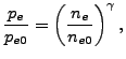
Collisionless plasmas are often modeled using fluid magnetohydrodynamics (MHD) models. However, the MHD fluid approximation is questionable when the gyroradius of the ions is large compared to the spatial region that is studied. On the other hand, kinetic models that discretize the full velocity space, or full particle in cell (PIC) models that treat ions and electrons as particles, are computationally very expensive. For problems where the time scales and spatial scales of the ions are of interest, hybrid models provide a compromise. In such models, the ions are treated as discrete particles, while the electrons are treated as a (often massless) fluid. This mean that the time scales and spatial scales of the electrons do not need to be resolved, and enables applications such as modeling of the solar wind interaction with planets. For a detailed discussion of different plasma models, see Ledvina et al. (2008).

21.1.2.1 The hybrid equations

In the hybrid approximation, ions are treated as particles, and electrons as a massless fluid. In what follows we use SI units. We have $N_I$ ions at positions $\mathbf{r}_i(t)$ [m] with velocities $\mathbf{v}_i(t)$ [m/s], mass $m_i$ [kg] and charge $q_i$ [C], $i=1,\ldots,N_I$. By spatial averaging we can define the charge density $\rho_I(\mathbf{r},t)$ [Cm$^{-3}$] of the ions, their average velocity $\mathbf{u}_I(\mathbf{r},t)$ [m/s], and the corresponding current density $\mathbf{J}_I(\mathbf{r},t)=\rho_I\mathbf{u}_I$ [Cm$^{-2}$s$^{-1}$]. Electrons are modelled as a fluid with charge density $\rho_e(\mathbf{r},t)$, average velocity $\mathbf{u}_e(\mathbf{r},t)$, and current density $\mathbf{J}_e(\mathbf{r},t)=\rho_e\mathbf{u}_e$. The electron number density is $n_e=-\rho_e/e$, where $e$ is the elementary charge. If we assume that the electrons are an ideal gas, then $p_e=n_ekT_e$, so the pressure is directly related to temperature ($k$ is Boltzmann's constant).

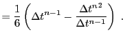
The trajectories of the ions are computed from the Lorentz force,

$$\dfrac{d\mathbf{r}_i}{dt} = \mathbf{v}_i, \quad \dfrac{d\mathbf{v... ... \left( \mathbf{E}+\mathbf{v}_i\times\mathbf{B} \right), \quad i=1,\ldots,N_I$$

where $\mathbf{E}=\mathbf{E}(\mathbf{r},t)$ is the electric field, and $\mathbf{B}=\mathbf{B}(\mathbf{r},t)$ is the magnetic field. The electric field is given by

$$\mathbf{E} = \dfrac{1}{\rho_I} \left( -\mathbf{J}_I\times\mathbf{... ...hbf{B} - \nabla p_e \right) + \eta \mathbf{J} - \eta_h \nabla^2 \mathbf{J},$$

where $\rho_I$ is the ion charge density, $\mathbf{J}_I$ is the ion current, $p_e$ is the electron pressure, $\mu_0=4\pi\cdot10^{-7}$ is the magnetic constant, $\mathbf{J}=\mu_0^{-1}\nabla\times\mathbf{B}$ is the current, and $\eta_h$ is a hyperresistivity. Here we assume that $p_e$ is adiabatic. Then the relative change in electron pressure is related to the relative change in electron density by

$$\frac{p_e}{p_{e0}} = \left( \frac{n_e}{n_{e0}} \right)^{\gamma} ,$$

where the zero subscript denote reference values (here the initial values at $t=0$). Then Faraday's law is used to advance the magnetic field in time,

$$\frac{\displaystyle\partial\mathbf{B}}{\displaystyle\partial t} = -\nabla\times\mathbf{E}.$$

21.1.2.2 A cell-centered finite difference hybrid PIC solver

We use a cell-centered representation of the magnetic field on a uniform grid. All spatial derivatives are discretized using standard second order finite difference stencils. Time advancement is done by a predictor-corrector leapfrog method with subcycling of the field update, denoted cyclic leapfrog (CL) by Matthew (1994). An advantage of the discretization is that the divergence of the magnetic field is zero, down to round off errors. The ion macroparticles (each representing a large number of real particles) are deposited on the grid by a cloud-in-cell method (linear weighting), and interpolation of the fields to the particle positions are done by the corresponding linear interpolation. Initial particle positions are drawn from a uniform distribution, and initial particle velocities from a Maxwellian distribution. Further details of the algorithm can be found in Holmström, M. (2012,2013) and references therein, where an extension of the solver that include inflow and outflow boundary conditions was used to model the interaction between the solar wind and the Moon. In what follows we describe the FLASH implementation of the hybrid solver with periodic boundary conditions.

21.1.2.3 Hybrid solver implementation

The two basic operations needed for a PIC code are provided as standard operations in FLASH:

• Deposit charges and currents onto the grid: call Grid_mapParticlesToMesh()
• Interpolate fields to particle positions: call Grid_mapMeshToParticles()

At present the solver is restricted to a Cartesian uniform grid, since running an electromagnetic particle code on an adaptive grid is not straightforward. Grid refinement/coarsening must be accompanied by particle split/join operations. Also, jumps in the cell size can lead to reflected electromagnetic waves.

The equations are stated in SI units, so all parameters should be given in SI units, and all output will be in SI units. The initial configuration is a spatial uniform plasma consisting of two species. The first species, named pt_picPname_1 consists of particles of mass pt_picPmass_1 and charge pt_picPcharge_1. The initial (at $t=0$) uniform number density is pt_picPdensity_1, and the velocity distribution is Maxwellian with a drift velocity of (pt_picPvelx_1, pt_picPvely_1, pt_picPvelz_1), and a temperature of pt_picPtemp_1. Each model macro-particle represents many real particles. The number of macro-particles per grid cell at the start of the simulation is set by pt_picPpc_1. So this parameter will control the total number of macro-particles of species 1 in the simulation.

All the above parameters are also available for a second species, e.g., pt_picPmass_2, which is initialized in the same way as the first species.

Table: Runtime parameters for the hybrid solver. Initial values are at $t=0$. For each parameter for species 1, there is a corresponding parameter for species 2 (named with 2 instead of 1), e.g., pt_picPvelx_2.

Variable	Type	Default	Description
pt_picPname_1	STRING	"H+"	Species 1 name
pt_picPmass_1	REAL	1.0	Species 1 mass, $m_i$ [amu]
pt_picPcharge_1	REAL	1.0	Species 1 charge, $q_i$ [e]
pt_picPdensity_1	REAL	1.0	Initial $n_I$ species 1 [m$^{-3}$]
pt_picPtemp_1	REAL	1.5e5	Initial $T_I$ species 1 [K]
pt_picPvelx_1	REAL	0.0	Initial $\mathbf{u}_I$ species 1 [m/s]
pt_picPvely_1	REAL	0.0
pt_picPvelz_1	REAL	0.0
pt_picPpc_1	REAL	1.0	Number of macro-particle of species 1 per cell
sim_bx	REAL	0.0	Initial $\mathbf{B}$ (at $t=0$) [T]
sim_by	REAL	0.0
sim_bz	REAL	0.0
sim_te	REAL	0.0	Initial $T_e$ [K]
pt_picResistivity	REAL	0.0	Resistivity, $\eta$ [$\Omega$ m]
pt_picResistivityHyper	REAL	0.0	Hyperresistivity, $\eta_h$
sim_gam	REAL	-1.0	Adiabatic exponent for electrons
sim_nsub	INTEGER	3	Number of CL B-field update subcycles (must be odd)
sim_rng_seed	INTEGER	0	Seed the random number generator (if $>0$)

The grid is initialized with the uniform magnetic field (sim_bx, sim_by, sim_bz).

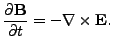
Now for grid quantities. The cell averaged mass density is stored in pden, and the charge density in cden. The magnetic field is represented by (grbx, grby, grbz). A background field can be set during initialization in (gbx1, gby1, gbz1). We then solve for the deviation from this background field. Care must be take so that the background field is divergence free, using the discrete divergence operator. The easiest way to ensure this is to compute the background field as the rotation of a potential. The electric field is stored in (grex, grey, grez), the current density in (grjx, grjy, grjz) , and the ion current density in (gjix, gjiy, gjiz). A resistivity is stored in gres, thus it is possible to have a non-uniform resistivity in the simulation domain, but the default is to set the resistivity to the constant value of sim_resistivity everywhere. For post processing, separate fields are stored for charge density and ion current density for species 1 and 2.

Table 21.4: The grid variables for the hybrid solver that are most important for a user. For each property for species 1, there is a corresponding variable for species 2 (named with 2 instead of 1), e.g., cde2.

Variable	Type	Description
cden	PER_VOLUME	Total charge density, $\rho$ [C/m$^3$]
grbx	GENERIC	Magnetic field, $\mathbf{B}$ [T]
grby	GENERIC
grbz	GENERIC
grex	GENERIC	Electric field, $\mathbf{E}$ [V/m]
grey	GENERIC
grez	GENERIC
grjx	PER_VOLUME	Current density, $\mathbf{J}$ [A/m$^2$]
grjy	PER_VOLUME
grjz	PER_VOLUME
gjix	PER_VOLUME	Ion current density, $\mathbf{J}_I$ [A/m$^2$]
gjiy	PER_VOLUME
gjiz	PER_VOLUME
cde1	PER_VOLUME	Species 1 charge density, $\rho_I$ [C/m$^3$]
jix1	PER_VOLUME	Species 1 ion current density, $\mathbf{J}_I$ [A/m$^2$]
jiy1	PER_VOLUME
jiz1	PER_VOLUME

Regarding particle properties. Each computational meta-particles is labeled by a positive integer, specie and has a mass and charge. As all FLASH particles they also each have a position $\mathbf{r}_i$=(posx, posy, posz) and a velocity $\mathbf{v}_i$=(velx, vely, velz). To be able to deposit currents onto the grid, each particle stores the current density corresponding to the particle, $\mathbf{J}_{Ii}$. For the movement of the particles by the Lorentz force, we also need the electric and magnetic fields at the particle positions, $\mathbf{E}(\mathbf{r}_i)$ and $\mathbf{B}(\mathbf{r}_i)$, respectivly.

Table 21.5: Important particle properties for the hybrid solver. Note that this is for the computational macro-particles.

Variable	Type	Description
specie	REAL	Particle type (an integer number 1,2,3,...)
mass	REAL	Mass of the particle, $m_i$ [kg]
charge	REAL	Charge of the particle, $q_i$ [C]
jx	REAL	Particle ion current, $\mathbf{J}_{Ii}=q_i\mathbf{v}_i$ [A m]
jy	REAL
jz	REAL
bx	REAL	Magnetic field at particle, $\mathbf{B}(\mathbf{r}_i)$ [T]
by	REAL
bz	REAL
ex	REAL	Electric field at particle, $\mathbf{E}(\mathbf{r}_i)$ [V/m]
ey	REAL
ez	REAL

Regarding the choice of time step. The timestep must be constant, $\Delta t=$dtinit = dtmin = dtmax, since the leap frog solver requires this. For the solution to be stable the time step, $\Delta t$, must be small enough. We will try and quantify this, and here we asume that the grid cells are cubes, $\Delta x=\Delta y=\Delta z$, and that we have a single species plasma.

First of all, since the time advancement is explicit, there is the standard CFL condition that no particle should travel more than one grid cell in one time step, i.e. $\Delta t$max$_i(\vert\mathbf{v}_i\vert) < \Delta x$. This time step is printed to standard output by FLASH (as dt_Part), and can thus be monitored.

Secondly, we also have an upper limit on the time step due to Whistler waves (Pritchett 2000),

$$\Delta t < \frac{ \Omega_i^{-1} }{\pi} \left( \frac{\Delta x}{\de... ...)^2, \qquad \delta_i = \frac{1}{\vert q_i\vert} \sqrt{\frac{m_i}{\mu_0 n}},$$

where $\delta_i$ is the ion inertial length, and $\Omega_i=\vert q_i\vert B/m_i$ is the ion gyrofrequency.

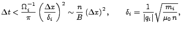
Finally, we also want to resolve the ion gyro motion by having several time steps per gyration. This will only put a limit on the time step if, approximately, $\Delta x > 5 \delta_i$, and we then have that $\Delta t < \Omega_i^{-1}$.

All this are only estimates that does not take into account, e.g., the initial functions, or the subcycling of the magnetic field update. In practice one can just reduce the time step until the solution is stable. Then for runs with different density and/or magnetic field strength, the time step will need to be scaled by the change in $n_{I}/B$, e.g., if $n_{I}$ is doubled, $\Delta t$ can be doubled. The factor $\left(\Delta x\right)^2$ implies that reducing the cell size by a factor of two will require a reduction in the time step by a factor of four.

21.1.3 Passive Particles

Passive particles may be moved using one of several different methods available in FLASH4. With the exception of Midpoint, they are all single-step schemes. The methods are either first-order or second-order accurate, and all are explicit, as described below. In all implementations, particle velocities are obtained by mapping grid-based velocities onto particle positions as described in Sec:Particles Mapping.

Numerically solving Equation (21.1) for passive particles means solving a set of simple ODE initial value problems, separately for each particle, where the velocities ${\bf v}_i$ are given at certain discrete points in time by the state of the hydrodynamic velocity field at those times. The time step is thus externally given and cannot be arbitrarily chosen by a particle motion ODE solver^21.1. Statements about the order of a method in this context should be understood as referring to the same method if it were applied in a hypothetical simulation where evaluations of velocities ${\bf v}_i$ could be performed at arbitrary times (and with unlimited accuracy). Note that FLASH4 does not attempt to provide a particle motion ODE solver of higher accuracy than second order, since it makes little sense to integrate particle motion to a higher order than the fluid dynamics that provide its inputs.

In all cases, particles are advanced in time from $t^n$ (or, in the case of Midpoint, from $t^{n-1}$) to $t^{n+1} = t^n + \Delta t^n$ using one of the difference equations described below. The implementations assume that at the time when Particles_advance is called, the fluid fields have already been updated to $t^{n+1}$, as is the case with the Driver_evolveFlash implementations provided with FLASH4. A specific implementation of the passive portion of Particles_advance is selected by a setup option such as -with-unit=Particles/ParticlesMain/passive/Euler, or by specifying something like REQUIRES Particles/ParticlesMain/passive/Euler in a simulation's Config file (or by listing the path in the Units file if not using the -auto configuration option). Further details are given is Sec:ParticlesUsing below.

• Forward Euler (Particles/ParticlesMain/passive/Euler). Particles are advanced in time from $t^n$ to $t^{n+1} = t^n + \Delta t^n$ using the following difference equation:

  $${\bf x}_i^{n+1} = {\bf x}_i^n + {\bf v}_i^n\Delta t^n \quad.$$ (21.7)

  
  
  Here ${\bf v}_i^n$ is the velocity of the particle, which is obtained using particle-mesh interpolation from the grid at $t=t^n$.

  Note that this evaluation of ${\bf v}_i^n$ cannot be deferred until the time when it is needed at $t=t^{n+1}$, since at that point the fluid variables have been updated and the velocity fields at $t=t^n$ are not available any more. Particle velocities are therefore interpolated from the mesh at $t=t^n$ and stored as particle attributes. Similar concerns apply to the remaining methods but will not be explicitly mentioned every time.

• Two-Stage Runge-Kutta (Particles/ParticlesMain/passive/RungeKutta). This 2-stage Runge-Kutta scheme is the preferred choice in FLASH4. It is also the default which is compiled in if particles are included in the setup but no specific alternative implementation is requested. The scheme is also known as Heun's Method:
  

  $${\bf x}_i^{n+1} = {\bf x}_i^n + \frac{\Delta t^n}{2} \left[ {\bf v}_i^n + {\bf v}_i^{*,n+1} \right] \;,$$ (21.8)

  $$\hbox{where}\quad {\bf v}_i^{*,n+1} = {\bf v}({\bf x}_i^{*,n+1},t^{n+1}) \;,$$

  $${\bf x}_i^{*,n+1} = {\bf x}_i^n + \Delta t^n {\bf v}_i^n \quad.$$

  
  Here ${\bf v}({\bf x},t)$ denotes evaluation (interpolation) of the fluid velocity field at position $\bf x$ and time $t$; ${\bf v}_i^{*,n+1}$ and ${\bf x}_i^{*,n+1}$ are intermediate results ^21.2; and ${\bf v}_i^n = {\bf v}({\bf x}_i^{n},t^{n})$ is the velocity of the particle, obtained using particle-mesh interpolation from the grid at $t=t^n$ as usual.

• Midpoint (Particles/ParticlesMain/passive/Midpoint). This Midpoint scheme is a two-step scheme. Here, the particles are advanced from time $t^{n-1}$ to $t^{n+1} = t^{n-1} + \Delta t^{n-1} + \Delta t^{n}$ by the equation

  $${\bf x}_i^{n+1} = {\bf x}_i^{n-1} + {\bf v}_i^{n}(\Delta t^{n-1} + \Delta t^{n}) \quad.$$ (21.9)

  
  
  The scheme is second order if $\Delta t^n = \Delta t^{n-1}$.

  To get the scheme started, an Euler step (as described for passive/Euler) is taken the first time Particles/ParticlesMain/passive/Midpoint/pt_advancePassive is called.

  The Midpoint alternative implementation uses the following additional particle attributes:  
  

  PARTICLEPROP pos2PrevX REAL           # two previous x-coordinate
  PARTICLEPROP pos2PrevY REAL           # two previous y-coordinate
  PARTICLEPROP pos2PrevZ REAL           # two previous z-coordinate
  

• Estimated Midpoint with Correction (Particles/ParticlesMain/passive/EstiMidpoint2). The scheme is second order even if $\Delta t^n = \Delta t^{n+1}$ is not assumed. It is essentially the EstiMidpoint or “Predictor-Corrector” method of previous releases, with a correction for non-constant time steps by using additional evaluations (at times and positions that are easily available, without requiring more particle attributes).

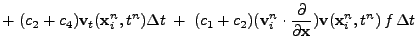
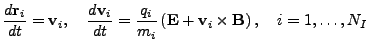
  Particle advancement follows the equation

  $${\bf x}_i^{n+1} = {\bf x}_i^n + {{\Delta t}}^n {\bf v}_i^{\mathrm{comb}}\;,$$ (21.10)

  
  
  where

  $${\bf v}_i^{\mathrm{comb}}= c_1 {\bf v}({\bf x}_i^{*,n+\frac12},t... ...n+1}) + c_3 {\bf v}({\bf x}_i^{n},t^{n}) + c_4 {\bf v}({\bf x}_i^{n},t^{n+1})$$ (21.11)

  
  
  is a combination of four evaluations (two each at the previous and the current time),

  $${\bf x}_i^{*,n+\frac12}= {\bf x}_i^n + \frac12 \Delta t^{n-1} {\bf v}_i^n$$

  
  
  are estimated midpoint positions as before in the Estimated Midpoint scheme, and the coefficients
  

  $$c_1 = c_1({\Delta t}^{n-1},{\Delta t}^n)\;,$$

  $$c_2 = c_2({\Delta t}^{n-1},{\Delta t}^n)\;,$$

  $$c_3 = c_3({\Delta t}^{n-1},{\Delta t}^n)\;,$$

  $$c_4 = \CD$$

  
  are chosen dependent on the change in time step so that the method stays second order when ${\Delta t}^{n-1} \neq {\Delta t}^n$.

  Conditions for the correction can be derived as follows: Let $\Delta t_{*}^{n} =\frac12 \Delta t^{n-1}$ the estimated half time step used in the scheme, let $t_{*}^{n+\frac12}=t^n + \Delta t_{*}^{n}$ the estimated midpoint time, and $t^{n+\frac12}=t^n + \frac12 \Delta t^{n}$ the actual midpoint of the $[t^n,t^{n+1}]$ interval. Also write ${\bf x}_i^{{\mathrm{E}},n+\frac12}= {\bf x}_i^{n}+ \frac12 \Delta t^{n}{\bf v}_i^{n}$ for first-order (Euler) approximate positions at the actual midpoint time $t^{n+\frac12}$, and we continue to denote with ${\bf x}_i^{*,n+\frac12}$ the estimated positions reached at the estimated mipoint time $t_{*}^{n+\frac12}$.

  Assuming reasonably smooth functions ${\bf v}({\bf x},t)$, we can then write for the exact value of the velocity field at the approximate positions evaluated at the actual midpoint time

  $${\bf v}({\bf x}_i^{{\mathrm{E}},n+\frac12},t^{n+\frac12}) = {\bf ... ...) {\bf v}({\bf x}_i^{n},t^{n})\frac12 \Delta t^{n}+ O((\frac12 \Delta t^{n})^2)$$ (21.12)

  
  
  by Taylor expansion. It is known that the propagation scheme $\widetilde{{\bf x}}_i^{n+1}={\bf x}_i^{n}+{\bf v}({\bf x}_i^{{\mathrm{E}},n+\frac12},t^{n+\frac12}) {\Delta t}$ using these velocities is second order (this is known as the modified Euler method).

  On the other hand, expansion of (21.11) gives
  

  $${\bf v}_i^{\mathrm{comb}} = (c_1+c_2+c_3+c_4) {\bf v}({\bf x}_i^{n},t^{n})$$

  $$+\; (c_2+ c_4) {\bf v}_t({\bf x}_i^{n},t^{n}) {\Delta t}\;+\; (c_... ...frac{\partial}{\partial {\bf x}}) {\bf v}({\bf x}_i^{n},t^{n}) \Delta t_{*}^{n}$$

  $$\quad + \mbox{higher order terms in ${\Delta t}$ and $\Delta t_{*}^{n} $.}$$

  
  After introducing a time step factor $f$ defined by $\Delta t_{*}^{n} = f {\Delta t}^{n}$, this becomes
  

  $${\bf v}_i^{\mathrm{comb}} = (c_1+c_2+c_3+c_4) {\bf v}({\bf x}_i^{n},t^{n})$$ (21.13)

  $$+\; (c_2+ c_4) {\bf v}_t({\bf x}_i^{n},t^{n}) {\Delta t}\;+\; (c_... ...\frac{\partial}{\partial {\bf x}}) {\bf v}({\bf x}_i^{n},t^{n}) f {\Delta t}$$

  $$\quad + \; O(({\Delta t})^2)\quad.$$

  
  

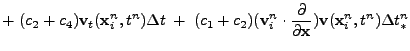  One can derive conditions for second order accuracy by comparing (21.13) with (21.12) and requiring that

  $${\bf v}_i^{\mathrm{comb}}= {\bf v}({\bf x}_i^{{\mathrm{E}},n+\frac12},t^{n+\frac12}) + O(({\Delta t})^2)\quad.$$ (21.14)

  
  
  It turns out that the coefficients have to satisfy three conditions in order to eliminate from the theoretical difference between numerical and exact solution all $O({\Delta t}^{n-1})$ and $O({\Delta t}^{n})$ error terms:
  

  $$c_1+c_2+c_3+c_4 = 1 \;,$$

  $$c_2+c_4 = \frac12 \mbox{(and thus also $c_1+c_3=\frac12$)} \;,$$

  $$c_1+c_2 = \frac{ {\Delta t}^n } { {\Delta t}^{n-1} } \quad.$$

  
  The provided implementation chooses $c_4=0$ (this can be easily changed if desired by editing in the code). All four coefficients are then determined:
  

  $$c_1 = \frac{ {\Delta t}^n } { {\Delta t}^{n-1} } - \frac12\;,$$

  $$c_2 = \frac12\;,$$

  $$c_3 = 1 - \frac{ {\Delta t}^n } { {\Delta t}^{n-1} }\;,$$

  $$c_4 = 0\quad.$$

  
  Note that when the time step remains unchanged we have $c_1=c_2=\frac12$ and $c_3=c_4=0$, and so (21.10) simplifies significantly.

  An Euler step, as described for passive/Euler in (21.7), is taken the first time when Particles/ParticlesMain/passive/EstiMidpoint2/pt_advancePassive is called and when the time step has changed too much. Since the integration scheme is tolerant of time step changes, it should usually not be necessary to apply the second criterion; even when it is to be employed, the criteria should be less strict than for an uncorrected EstiMidpoint scheme. For EstiMidPoint2 the timestep is considered to have changed too much if either of the following is true:

  $$\Delta t^{n} > \Delta t^{n-1}$$   and$$\quad \left\vert \Delta t^{n} - \Delta t^{n-1} \right\vert \geq {\tt pt\_dtChangeToleranceUp} \times \Delta t^{n-1}$$
  or
  $$\Delta t^{n} < \Delta t^{n-1}$$   and$$\quad \left\vert \Delta t^{n} - \Delta t^{n-1} \right\vert \geq {\tt pt\_dtChangeToleranceDown} \times \Delta t^{n-1},$$
  where pt_dtChangeToleranceUp and pt_dtChangeToleranceDown are runtime parameter specific to the EstiMidPoint2 alternative implementation.

  The EstiMidpoint2 alternative implementation uses the following additional particle attributes for storing the values of ${\bf x}_i^{*,n+\frac12}$ and ${\bf v}_i^{*,n+\frac12}$ between the Particles_advance calls at $t^n$ and $t^{n+1}$:  
  

  PARTICLEPROP velPredX REAL
  PARTICLEPROP velPredY REAL
  PARTICLEPROP velPredZ REAL
  PARTICLEPROP posPredX REAL
  PARTICLEPROP posPredY REAL
  PARTICLEPROP posPredZ REAL
  

The time integration of passive particles is tested in the ParticlesAdvance unit test, which can be used to examine the convergence behavior, see Sec:ParticlesUnitTest.