Next:
20.1 Introduction
Up:
V. Physics Units
Previous:
19.1 Diffuse Unit
Contents
Index
20
. Gravity Unit
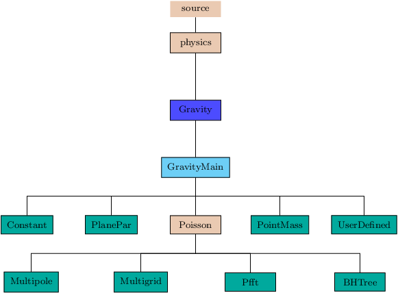
Figure 20.1:
The
Gravity
unit directory tree.
Subsections
20
.
1
Introduction
20
.
2
Externally Applied Fields
20
.
2
.
1
Constant Gravitational Field
20
.
2
.
2
Plane-parallel Gravitational field
20
.
2
.
3
Gravitational Field of a Point Mass
20
.
2
.
4
User-Defined Gravitational Field
20
.
3
Self-gravity
20
.
3
.
1
Coupling Gravity with Hydrodynamics
20
.
3
.
2
Tree Gravity
20
.
4
Usage
20
.
4
.
1
Tree Gravity Unit Usage
20
.
5
Unit Tests