Next: 20.4 Usage Up: 20. Gravity Unit Previous: 20.2 Externally Applied Fields Contents Index
| (20.3) | |||
Two algorithms are available for solving the Poisson equations: Gravity/GravityMain/Multipole and Gravity/GravityMain/Multigrid. The initialization routines for these algorithms are contained in the Gravity unit, but the actual implementations are contained below the Grid unit due to code architecture constraints.
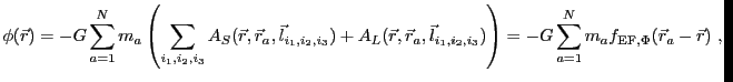
The multipole-based solver described in Sec:GridSolversMultipole for self gravity is appropriate for spherical or nearly-spherical mass distributions with isolated boundary conditions. For non-spherical mass distributions higher order moments of the solver must be used. Note that storage and CPU costs scale roughly as the square of number of moments used, so it is best to use this solver only for nearly spherical matter distributions.
The multigrid solver described in Sec:GridSolversMultigrid is appropriate for general mass distributions and can solve problems with more general boundary conditions.
The tree solver described in 8.10.2.4 is appropriate for general mass distributions and can solve problems with both isolated and periodic boundary conditions set independently in individual directions.
The gravitational field couples to the Euler equations only through the momentum and energy equations. If we define the total energy density as
| (20.4) |
For example, the PPM algorithm supplied with FLASH uses the following
update steps to obtain the momentum and energy in cell ![]() at timestep
at timestep
![]()
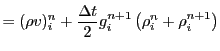 |
|||
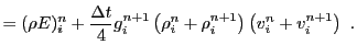 |
(20.5) |
Note that finite-volume schemes do
not retain explicit conservation of momentum and energy when gravity
source terms are added. Godunov schemes such as PPM, require an
additional step in order to preserve second-order time accuracy. The
gravitational acceleration component ![]() is fitted by interpolants along
with the other state variables, and these interpolants are used to
construct characteristic-averaged values of
is fitted by interpolants along
with the other state variables, and these interpolants are used to
construct characteristic-averaged values of ![]() in each cell. The
velocity states
in each cell. The
velocity states
![]() and
and
![]() , which are used as
inputs to the Riemann problem solver, are then corrected to account
for the acceleration using the following expressions
, which are used as
inputs to the Riemann problem solver, are then corrected to account
for the acceleration using the following expressions
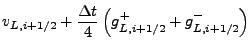 |
|||
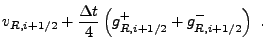 |
(20.6) |
The Tree implementation of the gravity unit in physics/Gravity/GravityMain/Poisson/BHTree is meant to be used together with the tree solver implementation Grid/GridSolvers/BHTree/Wunsch. It either calculates the gravitational potential field which is subsequently differentiated in subroutine Gravity_accelOneRow to obtain the gravitational acceleration, or it calculates the gravitational acceleration directly. The latter approach is more accurate, because the error due to numerical differentiation is avoided, however, it consumes more memory for storing three components of the gravitational acceleration. The direct acceleration calculation can be switched on by specifying bhtreeAcc=1 as a command line argument of the setup script.
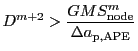
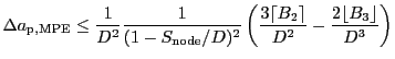
The gravity unit provides subroutines for building and walking the tree called by the tree solver. In this version, only monopole moments (node masses) are used for the potential/acceleration calculation. It also defines new multipole acceptance criteria (MACs) that estimate the error in gravitational acceleration of a contribution of a single node to the potential (hereafter partial error) much better than purely geometrical MAC defined in the tree solver. They are: (1) the approximate partial error (APE), and (2) the maximum partial error (MPE). The first one is based on an assumption that the partial error is proportional to the multipole moment of the node. The node is accepted for calculation of the potential if
 |
(20.7) |
The second MAC (maximum partial error, MPE) calculates the error in acceleration
of a single node contribution
![]() according to formula 9
from Salmon&Warren (1994; see this paper for details):
according to formula 9
from Salmon&Warren (1994; see this paper for details):
 |
(20.8) |
During the tree walk, subroutine Gravity_bhNodeContrib adds contributions of tree nodes to the gravitational potential or acceleration fields. In case of the potential, the contribution is
 |
(20.9) |
| (20.10) |
 |
(20.11) |
| (20.12) |
Boundary conditions can be isolated or periodic, set independently for each
direction. If they are periodic at least in one direction, the Ewald method is
used for the potential calculation (Ewald, P. P., 1921, Ann. Phys. 64, 253).
The original Ewald method is an efficient method for computing gravitational
field for problems with periodic boundary conditions in three directions. Ewald
speeded up evaluation of the gravitational potential by splitting it into two parts,
![]() (
(![]() is an
arbitrary constant) and then by applying Poisson summation formula on erfc
terms, gravitational field at position
is an
arbitrary constant) and then by applying Poisson summation formula on erfc
terms, gravitational field at position ![]() can be written in the form
can be written in the form
The gravity unit allows also to use a static external gravitational field read from file. In this version, the field can be either spherically symmetric or planar being only a function of the z-coordinate. The external field file is a text file containing three columns of numbers representing the coordinate, the potential and the acceleration. The coordinate is the radial distance or z-distance from the center of the external field given by runtime parameters. The external field if mapped to a grid using a linear interpolation each time the gravitational acceleration is calculated (in subroutine Gravity_accelOneRow).