43.5 Performance results

We present some performance results for each of the multithreaded FLASH units. It is important to note that the multithreaded speedup of each unit is not necessarily representative of a full application because a full application spends time in units which are not (currently) threaded, such as Paramesh, Particles and I/O.

All of the experiments are run on Eureka, a machine at Argonne National Laboratory, which contains 100 compute nodes each with 2 x quad-core Xeon w/32GB RAM. We make use of 1 node and run FLASH with 1 MPI task and 1-8 OpenMP threads.

43.5.1 Multipole solver

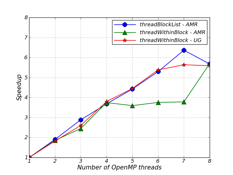
We tested the MacLaurin Spheroid problem described in Section 35.3.4 with the new Multipole solver described in Section 8.10.2.2 using three FLASH applications: one with Paramesh and block list threading, one with Paramesh and within block threading and one with UG and within block threading. The FLASH setup lines are

 

./setup unitTest/Gravity/Poisson3 -auto -3d -maxblocks=600 -opt  +pm4dev +newMpole +noio threadBlockList=True timeMultipole=True


./setup unitTest/Gravity/Poisson3 -auto -3d -maxblocks=600 -opt  +pm4dev +newMpole +noio threadWithinBlock=True timeMultipole=True


./setup unitTest/Gravity/Poisson3 -auto -3d +ug -opt +newMpole +noio  threadWithinBlock=True timeMultipole=True -nxb=64 -nyb=64 -nzb=64

The effective resolution of the experiments are the same: the Paramesh experiments have lrefine_max=4 and blocks containing 8 internal cells along each dimension and the UG experiment has a single block containing 64 internal cells along each dimension. We add the setup variable timeMultipole to include a custom implementation of Gravity_potentialListOfBlocks.F90 which repeats the Poisson solve 100 times.

Figure 43.1: Speedup of the threaded Multipole solver in the Maclaurin Spheroid test problem.

The results in Figure 43.1 demonstrate multithreaded speedup for three different configurations of FLASH. The speedup for the AMR threadWithinBlock application is about the same for 4 threads as it is for 5,6 and 7 threads. This is because we parallelize only the slowest varying dimension with a static loop schedule and so some threads are assigned 64 cells per block whilst others are assigned 128 cells per block. We do not see the same issue with the UG threadWithinBlock application because the greater number of cells per block avoids the significant load imbalance per thread.

43.5.2 Helmholtz EOS

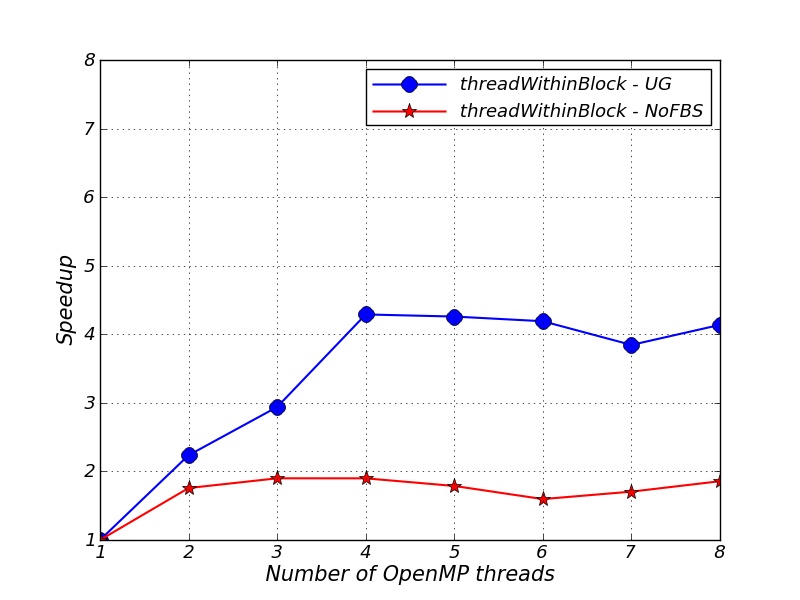
We tested the Helmholtz EOS unit test described in Section 17.7 with a UG and a NoFBS FLASH application. The FLASH setup lines are

 

./setup unitTest/Eos/Helmholtz -auto -3d +ug threadWithinBlock=True  timeEosUnitTest=True +noio


./setup unitTest/Eos/Helmholtz -auto -3d +nofbs threadWithinBlock=True  timeEosUnitTest=True +noio

The timeEosUnitTest setup variable includes a version of Eos_unit.F90 which calls Eos_wrapped 30,000 times in MODE_DENS_TEMP.

Figure 43.2: Speedup of the threaded Helmholtz EOS in the EOS unit test.

The results in Figure 43.2 show that the UG version gives better speedup than the NoFBS version. This is most likely because the NoFBS version contains dynamic memory allocation / deallocation within Eos_wrapped.

The UG application does not show speedup beyond 4 threads. This could be because the work per thread for each invocation of Eos_wrapped is too small, and so it would be interesting to re-run this exact test with blocks larger than $8 \times 8 \times 8$ cells. Unfortunately the Helmholtz EOS unit test does not currently support larger blocks - this is a limitation of the Helmholtz EOS unit test and not Helmholtz EOS.

43.5.3 Sedov

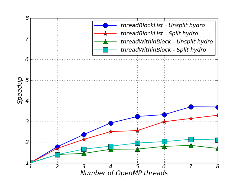
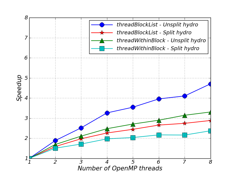
We ran 2d and 3d multithreaded versions of the standard Sedov simulation described in Section 35.1.4. We tested both split and unsplit hydrodynamic solvers and both threadBlockList and threadWithinBlock threading strategies. The 2d setup lines are

 

./setup Sedov -2d -auto +pm4dev -parfile=coldstart_pm.par  -nxb=16 -nyb=16 threadBlockList=True +uhd


./setup Sedov -2d -auto +pm4dev -parfile=coldstart_pm.par  -nxb=16 -nyb=16 threadWithinBlock=True +uhd


./setup Sedov -2d -auto +pm4dev -parfile=coldstart_pm.par  -nxb=16 -nyb=16 threadBlockList=True


./setup Sedov -2d -auto +pm4dev -parfile=coldstart_pm.par  -nxb=16 -nyb=16 threadWithinBlock=True

and the 3d setup lines are

 

./setup Sedov -3d -auto +pm4dev -parfile=coldstart_pm_3d.par  +cube16 threadBlockList=True +uhd


./setup Sedov -3d -auto +pm4dev -parfile=coldstart_pm_3d.par  +cube16 threadWithinBlock=True +uhd


./setup Sedov -3d -auto +pm4dev -parfile=coldstart_pm_3d.par  +cube16 threadBlockList=True


./setup Sedov -3d -auto +pm4dev -parfile=coldstart_pm_3d.par  +cube16 threadWithinBlock=True

The results are shown in Figures 43.3 and 43.4. The speedup graph is based on times obtained from the “hydro” timer label in the FLASH log file.

Figure 43.3: Speedup of the threaded hydrodynamic solvers in a 2d Sedov test.

Figure 43.4: Speedup of the threaded hydrodynamic solvers in a 3d Sedov test.

Part of the reason for loss of speedup in Figures 43.3 and 43.4 is that the hydrodynamic solvers in FLASH call Paramesh subroutines to exchange guard cells and conserve fluxes. Paramesh is not (yet) multithreaded and so we call these subroutines with a single thread. All other threads wait at a barrier until the single thread has completed execution.

The unsplit hydro solver has one guardcell fill per hydro timestep and the split hydro solver has NDIM guardcell fills per hydro timestep (one per directional sweep). The extra guardcell fills are part of the reason that the split applications generally give worse speedup than the unsplit applications.

43.5.4 LaserSlab

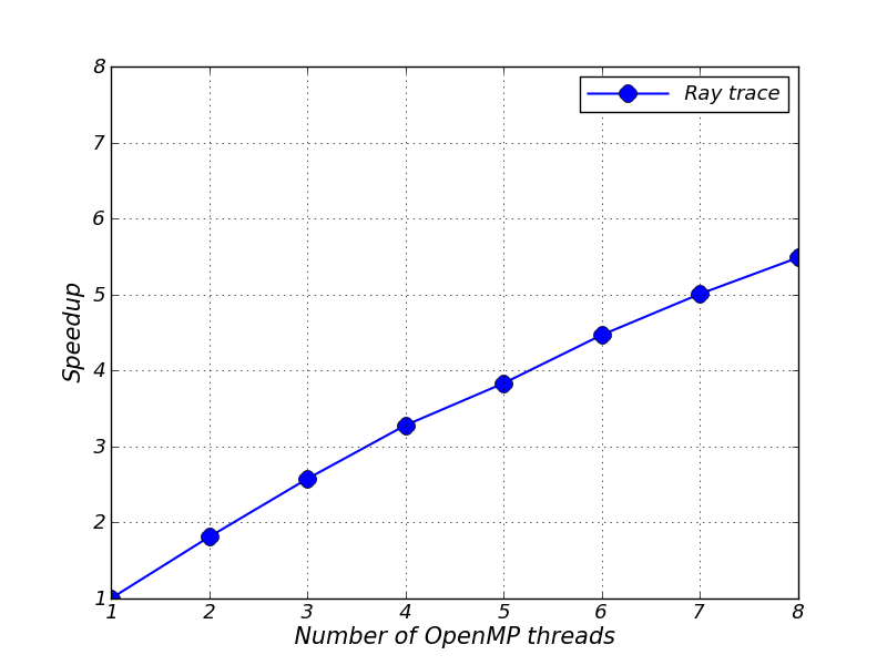
We finish with a scaling test for the ray trace in the energy deposition unit. We setup the LaserSlab simulation described in Section 35.7.5 with the additional setup option threadRayTrace=True. The setup line and our parameter modifications are

 

./setup LaserSlab -2d -auto +pm4dev -geometry=cylindrical  -nxb=16 -nyb=16 +mtmmmt +laser +mgd +uhd3t species=cham,targ  mgd_meshgroups=6 -without-unit=flashUtilities/contiguousConversion  -without-unit=flashUtilities/interpolation/oneDim  -parfile=coldstart_pm_rz.par threadRayTrace=True +noio


ed_maxRayCount = 80000
ed_numRays_1 =  50000
nend = 20

The speedup is calculated from times obtained from the “Transport Rays” label in the FLASH log file and the speedup graph is shown in Figure 43.5. The timer records how long it takes to follow all rays through the complete domain during the timestep. As an aside we remove the flashUtilities units in the setup line to keep the number of line continuation characters in a setup script generated Fortran file less than 39. This is just a workaround for picky compilers; another strategy could be a compiler option that allows compilation of Fortran files containing more than 39 continuation characters.

Figure 43.5: Speedup of the energy deposition ray trace in the LaserSlab test.